Introduction

The properties of a turbulent flow can be analyzed by measuring the dispersion of passive particles or tracers. Based on this idea, several studies have examined the turbulent character of the oceans and the atmosphere by releasing a number of drifters or substances that are advected by the flow (^{Griffa et al. 1995}). Surface and subsurface drifters (the latter reaching depths of hundreds and even a few thousand meters) are commonly used to study oceanic dispersion at different temporal and spatial scales (^{LaCasce, 2008}). Since the 1960s, controlled dye-release experiments in the ocean mixed layer have been carried out (^{Okubo, 1971}). In the atmosphere, constant level balloons advected by the winds at different heights (e. g. the 200 mb-level) are often used to study their dispersion (^{LaCasce, 2010}). Once the data set has been collected, either in a single campaign or during several observational periods, the statistical properties of the dispersion are calculated.

Different statistical analysis can be performed with the position and velocity components, such as single-particle statistics (with individual drifters) or two-particle statistics (with drifter pairs; see ^{LaCasce, 2008}). A fundamental tool for this purpose are the probability density functions (PDFs) of positions and velocities, which allow the calculation of statistical moments of the data records (e. g. dispersion, skewness, kurtosis).

The velocity PDFs might have a Gaussian or a non-Gaussian shape, which indicates how to parameterize dispersive properties of the turbulent flow. For instance, the evolution of a tracer concentration is often modeled with an advection-diffusion equation in an Eulerian framework, where the flow is decomposed into a large-scale flow, responsible for the advection, and a turbulent component associated with the diffusion (^{Griffa, 1996}). Then, the ‘eddy diffusivity’ associated with the small-scale motions is parameterized with Lagrangian data, that is, by calculating the statistical behavior of a number of particles advected by the flow. The generalized advection-diffusion model of ^{Davis (1987)} requires the velocity PDFs to be Gaussian or nearly-Gaussian. In order to apply this model, ^{Swenson and Niiler (1996)} computed the velocity PDFs from the California Current and reported a Gaussian shape in most of their samples. Surface velocities calculated from satellite altimetry also show a Gaussian distribution (^{Gille and Llewellyn-Smith, 2000}). However, other studies have shown that the PDFs can be strongly non-Gaussian for subsurface floats in the North Atlantic Ocean (^{Bracco et al., 2000}a; ^{LaCasce, 2005}) and in the surface of the Mediterranean Sea (^{Isern-Fontanet et al., 2006}). Such distributions are characterized by long tails, which indicate the presence of infrequent, but very energetic circulation events. In the ocean, these events are associated with intense mesoscale vortices and jets.

The shape of the velocity PDFs has been thoroughly studied in two-dimensional turbulent flows, where energetic coherent structures are formed due to the inverse energy cascade that characterizes this type of turbulence (^{Provenzale, 1999}; ^{Bracco et al., 2000b}). If the Reynolds number is moderate, and hence the vortices are relatively slow, the PDFs might be Gaussian or nearly-Gaussian. By contrast, for a large Reynolds number very intense vortices are generated and the PDFs might be clearly non-Gaussian (^{Bracco et al., 2000b}). Based on this, ^{Pasquero et al. (2001)} parameterized dispersive effects by using a suitable stochastic model that reproduces the non-Gaussian shape of the PDFs. Summarizing, transport processes can be very different depending on the shape of the velocity distributions, and it is therefore relevant to determine the PDFs in dispersion studies.

In this article we calculate single-particle statistics from a large set of surface drifters released in the southern Gulf of Mexico (hereafter GM). In particular, we estimate diffusivity scales and compare them with those reported in other regions. Afterwards we analyze the velocity PDFs and find that the distributions have extended wings, which represent infrequent, high energy velocity records (with respect to the mean). With this analysis we are able to identify the most energetic regions that generate the non-Gaussian distributions, and to show that these correspond to the semi-permanent cyclonic gyre in the Bay of Campeche and to the intense narrow flows along the western margin.

In previous studies we examined two-particle statistics (^{Zavala Sansón et al., 2017}a) and dispersion from localized areas regarded as point sources (^{Zavala Sansón et al., 2017b}), so the present work completes a series of Lagrangian analyses in the southern GM. These studies constitute an observational baseline for future observational and numerical Lagrangian studies in this region. One of the main motivations for gathering this information is to provide robust statistical results from a large drifter database that may shed some light on how to parameterize Lagrangian dispersion. For instance, operational numerical models that simulate particle dispersion can be evaluated by examining their ability to reproduce at least some of the statistics presented in these studies (PDFs, Lagrangian scales, dispersion curves).

The paper is organized as follows. The data set is briefly described in Drifter database section. Calcultions of single-particle statistics (mean fields, integral time scales and absolute dispersion) are shown in Results section. Afterwards, the velocity PDFs and the energetic circulations responsible for the non-Gaussian shape of the distributions are analyzed. Finally, in the last section, the results are discussed.

Drifter database

Lagrangian data were obtained during a long-term observational program in the southern GM, developed by the Mexican oil industry (PEMEX and CICESE, Mexico). The drifter database has been used to describe general features of the southern and western circulation of the GM (^{Pérez-Brunius et al., 2013}), and to estimate two-particle statistics (^{Zavala Sansón et al., 2017a},^b). It has also been used to examine the connectivity between the Bay of Campeche and the rest of the GM (^{Rodríguez-Outerelo, 2015}). Detailed information on the drifters’ performance and several pre-processing steps are described in those studies. Here a brief account of the results shown in the next section is presented.

Between September 2007 and September 2014, a total of 441 surface drifters (Far Horizon Drifters, Horizon Marine Inc.) were released by aircraft in different locations of the southern GM. The drifters consist of a cylindrical buoy attached to a parachute that serves as drogue at a nominal depth of 50 m when the buoy drifts in the water. It is estimated that the drifters effectively follow oceanic currents below the surface Ekman layer. The geographical positions were tracked with a GPS receiver recording hourly positions. The data were filtered and interpolated to regular 6 h intervals. On average, there were about 63 launches per year, and 5 or 6 per month. The average lifetime of the drifters is 62 days with a standard deviation of 47 days. The longest record was 218 days.

Most drifters were released near five preferential locations between 19^o and 20^o N, and 96^o and 93^o W (see detailed maps in ^{Zavala Sansón et al., 2017a},^b). Figure 1 shows the drifter trajectories up to 30 days, in order to illustrate their spatial distribution. The panels present the trajectories of 356 drifters starting from the preferential spots (panels a to e) and 85 drifters that started elsewhere (panel f). The first 15-day segments are colored differently than the subsequent sections.

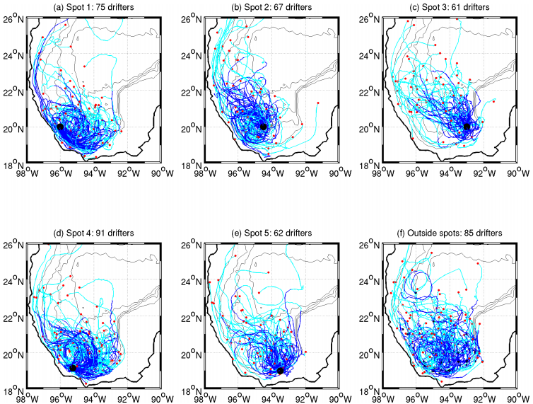
Figure 1 Trajectories of 441 drifters released in the southern GM. Panels (a) to (e) show the trajectories of 356 drifters released at five special locations denoted with a big black dot in each panel. 85 more drifters where released elsewhere (panel f). The maximum duration of the trajectories was 30 days. The first 15 days are colored in blue; subsequent days are colored in cyan. Small, black (red) dots indicate the initial (final) position of drifters. Topography contours (500, 1500, 2500 and 3500 m) are denoted with thin black lines. 

Most drifters were retained in the south during the first 15 days, many of them trapped in the Campeche gyre, the semi-permanent cyclonic circulation at the Bay of Campeche (^{Monreal-Gómez and Salas de León, 1997}; ^{Pérez-Brunius et al., 2013}). This is particularly clear at the western spots (panels a, b and d). When the drifters escape northwards during the subsequent 15 days, they do it preferentially along the western margin of the GM. On the eastern side, very few drifters were able to reach the Yucatan shelf, beyond 92.5^o W.

Results

Mean field

For the 84-month, 104232 drifter positions and velocities were recorded. The number of records in a regular grid of 0.25^o resolution is plotted in Figure 2a. Only geographical bins having a number of records larger than 30 were considered (^{Bracco et al., 2000a}). The number of records is greater in the southern part (below 22^o N), where most of the drifters were released. Note that some regions of the GM are sub-sampled, such as the eastern part and the Yucatan shelf. The reason is because drifters released at the southern GM barely transit over these regions. By interpolating the velocity records onto the grid (with mxn nodes) the mean velocity field (u^mn,v^mn) was generated, conformed by the zonal and meridional components, respectively (Figure 2b). A relevant feature is the cyclonic gyre at the Bay of Campeche, which reveals the extraordinary persistence in time of this structure. Another important feature is the northward flow along the western margin, between 22^o and 26 ^o N, which is associated with a northward advection of drifters observed in previous works (^{Pérez-Brunius et al., 2013}; ^{Zavala Sansón et al., 2017a},^b).

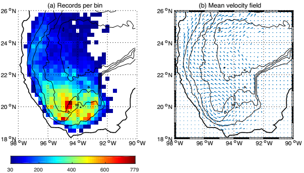
Figure 2 (a) Data records per geographical bin in a 0.25° 0.25° grid. Bins with less than 30 records are left blank. (b) Eulerian velocity field calculated from the mean records at each bin. Maximum velocity magnitude was 0.4 m/s. 

The kinetic energy field (per mass unit)

Emn=12umn2+vmn2 (1)

is shown in Figure 3a. The field is normalized with the mean value of the whole velocity records, E = 0.0624 m²/s². The highest values are concentrated at the western margin and at the northern side. Some areas in the southern and central regions are also very energetic (about 1.5 times the mean value). The variance of the velocity field is presented in Figure 3b. High values are found at the western coast, indicating the important variability of alongshore currents. In fact, even though the mean flow shows a south-to-north direction, the boundary flow can reverse its direction from north-to-south depending on the along-coast winds or due to the collision of mesoscale eddies with the shelf (^{Zavala-Hidalgo et al. 2003}; ^{Dubranna et al., 2011}; ^{Zavala Sansón et al., 2017a}).

Figure 3 (a) Kinetic energy field normalized with the mean value of the velocity records E=0.0624 m²/s². (b) Normalized variance of the velocity field. Bins with less than 30 records were left blank. 

Lagrangian scales and absolute dispersión

The drifter velocity components at time t are denoted as u_i (t), where i = 1,2 indicates the zonal and meridional directions, respectively. Lagrangian scales are calculated with residual velocities obtained by subtracting the Eulerian mean flow as the particles transit over geographical bins

uit=ui't-uimn. (2)

Then, the ‘memory’ of the drifter is calculated with the Lagrangian autocovariance function defined as (^{Provenzale, 1999})

Riiτ=limt→∞1T1σi2∫0Tui'(t)ui't+τdt, (3)

Where σi2 is the velocity variance and <*>=(1/N) Σ* indicates ensemble average over N particles. The Lagrangian integral time is formally defined as TiL=∫0∞Rii(τ)dτ. For a random process the integral converges as Rii(τ) drops to zero. In practice, the integral time is usually calculated by integrating the autocorrelation function up to the first zero crossing time t _Z (^{Poulain and Niiler, 1989}; ^{Zavala Sansón, 2015})

TiL=∫0tzRii(τ)dτ. (4)

Lagrangian length and diffusivity scales are defined as

Li=σiTiL, Ki=Li2TiL, (5)

where the velocity standard deviation <σ_i > is calculated at time TiL.

Figure 4 shows plots of the autocorrelation function for each velocity component (panel a), and the corresponding Lagrangian integral time (panel b). It is found that T1L~1.5 and T2L~1.5 days. The Lagrangian timescales are L₁~30 km and L₂~36 km. Diffusivity scales are K₁~6.9x10⁷ and K₂~8.8x10⁷ cm²/s.

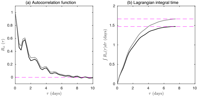
Figure 4 (a) Lagrangian velocity autocovariance for zonal (black line) and meridional (gray line) data. Horizontal dashed line indicates the zero. (b) Integral of the autocovariance calculated up to the first zero crossing for both components. Horizontal dashed lines indicate the value of the Lagrangian integral time. 

Absolute dispersion, which is based on the mean-squared separation of particles from their position at a reference time t₀ was calculated. Let x_i (t) be the position of particles in the i-direction at time t. Using N Lagrangian trajectories, absolute dispersion is (^{Provenzale, 1999})

Ai2-=xit-xit02. (6)

The asymptotic behavior for “short” times t≪TiL is the quadratic, ballistic regime in which dispersion grows as t². For “long” times t≫TiL dispersion grows linearly in time in a random-walk or standard dispersion regime (^{Taylor, 1921}). Absolute diffusion is defined as the temporal evolution of the dispersion

Ki=12ddtAi2-. (7)

For drifters with a long lifetime with respect to the integral timescale, it is possible to increase the number of degrees of freedom by making subdivisions of the trajectories in segments with a duration longer than TiL. This is a reasonable period after which every segment can be considered as an independent trajectory (^{Poulain and Niiler, 1989}). Using segments that are 10 days long, about 2500 ‘trajectories’ from the 441 original tracks were initially obtained.

Figure 5a presents the absolute dispersion components as a function of time. Between 0.25 and 3 days both components grow at the same rate, approximately. Within this time interval a quadratic curve is drawn, showing that the growth is nearly ballistic. At later times, between 5 and 60 days, the meridional component is approximately linear, indicating a random-walk regime. In contrast, the zonal component is limited by the western margin of the GM and hence its growth is slower than t. When using the 441 trajectories instead of the set of segments the results are very similar (not shown). Figure 5b shows the number of available segments as time evolves, about 2500 during the first 10 days, and up to 850 at day 60.

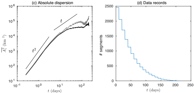
Figure 5 (a) Absolute dispersion components (zonal: black; meridional: gray) vs. time. For clarity, confidence intervals are not shown. The quadratic curve is drawn between 0.25 and 3 days, while the linear curve is drawn between 5 and 60 days. (b) Number of segments used to calculate absolute dispersion as a function of time. 

Probability density functions

The raw velocity PDFs using the velocity records without any modification is initially presented. Figures 6a-b shows the distributions in the zonal and meridional directions, respectively. Superposed to the empirical data a Gaussian distribution with the same standard deviation and zero mean for each component is plotted:

Pui=12π1/2σie-ui2/2σi2. (8)

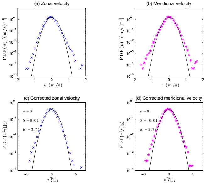
Figure 6 Velocity PDFs for (a) zonal (crosses) and (b) meridional (stars) records. Solid lines indicate the normal distribution (8). Corrected PDFs for both directions are shown in panels (c) and (d), respectively. Numbers in lower panels show the KS probability p, the skewness S and the kurtosis K. 

The extended tails suggest a non-Gaussian shape of the distributions. Considering that these deviations might be due to the presence of intense mean flows and not to turbulent dispersion, the velocity records are corrected in order to compensate the additional advection due to such motions. We follow the procedure used by ^{Bracco et al. (2000a)}, which consists of dividing the region of study in geographical bins (here the 0.25^o 0.25^o square grid considered above was used) discarding those with less than 30 velocity records. The Eulerian velocity is subtracted from each velocity record at the corresponding bin, as in equation (2), and the result is normalized with the standard deviation, so the new variables are ui'/σi. Finally, all the realizations are used to generate the re-scaled PDFs for the whole region. The results for the zonal and meridional velocity components are shown in Figures 6c-d. The skewness is close to zero in both cases and the kurtosis is nearly 3.8. Since the kurtosis of a normal distribution is 3, these results suggest that the corrected PDFs are not Gaussian (which is again evident from the extended tails).

In order to quantify the Gaussian part of these distributions, the Kolmogorov-Smirnov (KS) test was used (^{Beron-Vera and LaCasce, 2016}; ^{Zavala Sansón et al. 2017} PONER a o b). The samples must be statistically independent, which is achieved by taking data every integral time-scale (^{LaCasce, 2005}). Thus, only samples every 1.5 days were used, so the remaining records are 17231, approximately 1/6 of the total. The null hypothesis postulates that the distribution is sufficiently Gaussian when the KS probability p (associated with the maximum difference between the cumulative distribution of the empirical data and a Gaussian) is greater than the significance level α, chosen as 0.05. The KS probabilities for the zonal and meridional re-scaled PDFs are p = 2.3x10^-4 and p = 7.3x10^-6, respectively, and therefore the KS test confirms that these distributions are not Gaussian.

The extended tails of the PDFs are associated to infrequent but very energetic events that are mostly related with the presence of intense mesoscale features in the region. In order to show this, data subsets in which the most energetic records are subtracted were considered. The idea is to show that in such cases the PDFs tend to be Gaussian. The velocity records with “low” energy values are those whose energy is lower than sE, where E is the mean energy of the whole set (see Section 3.1) and the threshold is a positive real number. In Figures 7a-b the corrected PDFs for a low-energy subset with (16732 records) are presented, that is, the kinetic energy of each record is smaller than 3E. According to the KS test, both PDFs are Gaussian, because the KS probability p is larger than 0.05 and the corresponding kurtosis is nearly 3. This demonstrates that the low energy records have a normal PDF, and that the infrequent events in the tails of the whole distributions are indeed high energy records.

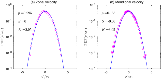
Figure 7 Low-energy velocity PDFs calculated with a threshold for (a) zonal (crosses) and (b) meridional (stars) records. Solid lines and numbers as in Figure 6. 

The KS test is applied to several low-energy subsets generated with different values. The results are presented in terms of the normalized energy of the records that are removed, that is, the high-energy fraction HEF. To define this number the total energy E_T of the whole set of records and the mean energy E were calculated. Then the threshold s was set and the total energy E_low (E_high) of the records whose energy is lower (greater) than sE was calculated. Since E_T = E_low + E_high then HEF is

HEF=EhighET=1-ElowET . (9)

The KS test is applied for HEF between 0 and 0.81, approximately, which corresponds with thresholds s = 40/q, where q = 1, 2, 3... 50.

Figures 8a-b present the KS probability and the kurtosis as a function of HEF for the zonal and meridional directions. For small HEF it is verified that the PDFs are non-Gaussian (p<0.05 and K>3). This is expected because the distributions are not Gaussian HEF = 0 when (i. e. when no records are removed, see Figures 6c-d). For intermediate HEF values, say between 0.1 and 0.6, the distributions become Gaussian ( p>0.05 and K~3). The first vertical dashed line at HEF~0.3 indicates the case of the PDFs shown in Figures 7a-b, where the threshold value is s = 3. The second and third vertical lines HEF~0.5 and 0.75) correspond to cases with s = 2 and s = 1, respectively. For larger HEF the PDFs become non-Gaussian again (p<0.05 and K<3 ), but now the reason is the reduced number of degrees of freedom as more and more records are subtracted (these later cases are of no interest).

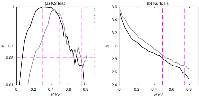
Figure 8 (a) Kolmogorov-Smirnov probability as a function of HEF defined in (9). The result of the test for the zonal (meridional) component is indicated with a black (gray) solid line. The horizontal dashed line represents the confidence level (0.05). The vertical dashed lines correspond to threshold values 3, 2 and 1 (from left to right). (b) Kurtosis of the distributions (line colors and styles as in previous panel). The value for a normal distribution (3) is indicated with a horizontal dashed line. 

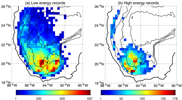
The geographical distribution of low and high energy records gives additional information, as shown in Figure 9 for the case with s = 2. The number of low energy records are found over almost the entire region, with maximum values at the Bay of Campeche (panel a). High energy records (panel b) are mainly located at the Bay of Campeche and a few more along the western boundary of the GM. This shows that very energetic records, responsible for the non-Gaussian form of the complete PDFs, are associated with the cyclonic gyre in Campeche and with the alongshore flow in the western margin.

Figure 9 (a) Low energy and (b) high energy records per geographical bin when using a threshold s=2 (see text). Bins with less than 30 records are left blank. 

Discussion

Lagrangian time, length and diffusivity scales were calculated from drifter records obtained during a 7-year period in the southern GM. The resulting diffusivities (from 6.9 to 8.8x10⁷ cm²/s) are now compared with similar calculations reported in previous studies for different regions of the GM.

^{Ohlmann and Niiler (2005)} made estimations for the Texas-Louisiana and northwest Florida shelves during the SCULP experiments performed during the 1990s. Diffusivities over the Texas-Louisiana shelf range from 6.4x10⁶ for inshore locations to 2.2x10⁷ cm²/s for offshore areas. Over the west Florida shelf, diffusivities were somewhat larger, ranging from 3.1 to 6.5x10⁷ cm²/s. Thus, diffusivities for the northern shelves of the GM are lower than the ones reported here, presumably because of the nearness to the coast.

More recently, ^{Mariano et al. (2016)} calculated Lagrangian statistics at coastal and offshore regions in the northeastern GM, using drifters from the GLAD experiment carried out in 2012. Horizontal diffusivity estimates near the coast and over the shelf are of order 10⁷ to 10⁸ cm²/s. In offshore areas under the influence of the Loop Current diffusivities mostly range between 1 and 4x10⁸ cm²/s, reaching peak values up to 2x10⁹ cm²/s. These large values (greater than those found in the southern GM) are apparently due to the considerable magnitude of the Loop Current and the subsequent formation of strong mesoscale eddies in eastern GM.

Using two-particle statistics, ^{Zavala Sansón et al. (2017a)} calculated relative diffusivities in the southern GM (relative diffusivity is two times the absolute diffusivity for large particle separations (^{LaCasce, 2008}). Their results range from 10⁶ cm²/s for small drifter separations (about 2 km) to 2x10⁸ cm²/s for larger separations (150-300 km). Recall, however, that these estimates are statistical values over a large set of drifters released at different times and locations. In other words, dispersion processes might change dramatically depending on the dominant circulation and this may lead to different dispersion scenarios, as described by ^{Zavala Sansón et al. (2017a},^b).

The examined shapes of the velocity PDFs, provide relevant information on the Lagrangian data and, consequently, on dispersion and diffusion properties. The velocity PDFs have a non-Gaussian shape characterized by long tails (with kurtoses of about 3.8). The non-Gaussian characteristic is associated with the presence of energetic circulation events, which generate the long tails of the distributions. This form of the PDFs has been discussed in dispersion studies for different oceanic regions (^{Bracco et al., 2000a}; ^{LaCasce, 2005}; ^{Isern-Fontanet et al., 2006}) and in numerical simulations of two-dimensional turbulence (^{Bracco et al., 2000b}; ^{Pasquero et al., 2001}).

One of the main mesoscale circulation features that characterizes the southern GM is the cyclonic gyre at the Bay of Campeche, which is clearly observed in the drifter trajectories and in the mean velocity field (Figures 1 and 2, respectively). It was shown that the PDFs become Gaussian when high-velocity records are removed, and that such a subset of records is indeed located in the area where the cyclonic gyre is usually formed (Figure 9). In other words, this circulation is apparently the main cause of the PDFs extended wings. Intense velocity records along the western margin were also found, associated with an alongshore flow frequently observed there (see e. g. ^{Zavala-Hidalgo et al., 2003}). When flowing northward, these currents have also been related with the arrival of Loop Current Eddies from the eastern GM (^{Pérez-Brunius et al., 2013}) and the consequent south-to-north dispersion of drifters (^{Zavala Sansón et al., 2017a},^b).

The identification of very energetic regions in the southern GM (with respect to the mean) points out that any parameterization has to take into account the influence of the intense circulations found there. Therefore diffusivity values calculated with the whole set of drifters might be underestimated in the regions with high energy records. In other words, high energy motions might generate anomalous, super-diffusive effects that cannot be parameterized with standard random-walk models (which generate Gaussian velocity distributions). The formulation of stochastic models that are able to reproduce non-Gaussian PDFs are scarce [see e. g. ^{Pasquero et al. (2001)} in the context of 2D turbulence] and such an approach should be followed in oceanic models.