


 nova página do texto(beta)
 Inglês (pdf)
 Artigo em XML
 Referências do artigo
 Enviar este artigo por email
 Citado por SciELO
  Similares em
SciELO
Similares em
SciELO 
 Permalink
Introduction
While modern computation capabilities allow the use of powerful methods (e.g. finite element and finite difference methods) based on data-intensive computing, the trade-off between parameterization and the non-uniqueness problem makes it difficult to find reliable solutions especially for underdetermined inverse problems. It is not always possible to add a priori information to constrain the inverse problem but sometimes a re-parameterization helps to reduce the non-uniqueness and allows obtaining simpler patterns. For example, measurements of deformation obtained by analyzing GPS time series have disclosed the existence of aseismic slip over active fault planes. However, frequently the number of GPS stations and the quality of data are not enough to adequately constrain the inverse problem, making it difficult to distinguish the details of slip distribution over the fault plane.
Okada’s (1985 and 1992) approach is usually applied to obtain displacement at the surface due to slip on a fault plane embedded in a half-space. For example, in a global inversion scheme (Iglesias et al., 2004) or a linear inversion method (Outerbridge et al., 2010) it is used to get the distribution of magnitude and direction of slip. There are different approaches to retrieve slip distribution over a fault plane (e.g.Radiguet et al., 2012, and 2016). Different methods using distinct approximations can provide equally good fits between data and synthetics with very different slip distributions (Mai and Beroza, 2000), which begs the question; which model is most realistic? To answer the question, Occam’s razor principle was invoked assuming that the simplest solution is the most appropriate. Therefore, a modified version of a frequency domain scheme was used to find kinematic parameters from displacement records (Cotton and Campillo, 1995) to retrieve slip within a fault plane at depth. Re-parameterization was performed by introducing slip only on simple geometrical patches within the fault plane. This is a restriction in which slip is distributed symmetrically within each ellipse, reducing the model parameters and therefore the number of model solutions. Furthermore, the computational time and non-uniqueness of the problem are reduced by this simplification. A simulated annealing inversion procedure was used to search for the best model parameters, as this procedure has been proven effective to explore a set of models and find a good solution in a complex misfit space (e.g.Kirkpatrick et al., 1983; Iglesias et al., 2001).
The suggested approach requires a calculation of the predicted displacement at each GPS station, due to a unitary force on each sub-fault; reference to these displacements will be as transfer functions (TF). One of the main objectives of this work is to set up a library of TF in order to use them in future slow slip events in the region. As the fault plane geometry will not change with time, the functions for every station could be readily used for impending SSE.
The Guerrero Pacific coast is an over 400 km long, active seismic region, within the Mexican Subduction Zone (MSZ). This region has been intensively studied because its NW part has been defined as a mature ~100 km length seismic gap (Singh et al., 1981) which has not produced any large earthquake since 1911. Several important cities in central Mexico were strongly affected by earthquakes occurred in the MSZ (e.g. 1911: M~7.5, 1957: 7.8, 1985: 8.0, 1995: 7.3, etc.). The first permanent GPS station deployed in the region began to operate early 1997 and at the beginning of 1998 a signal corresponding to a transient displacement was recorded (Lowry et al., 2001), later attributed to a slow slip event. Since then, the GPS networks have grown gradually and have recorded slow slip events with different complexity, about every 4 years. Slow slip events could have an important role in the seismic cycle, not only because slip may have reached the seismogenic (coupled zone) part of the subduction interface (Graham et al., 2015) but also because they may trigger large magnitude subduction thrust earthquakes (e.g.Graham et al.; 2014; Radiguet et al., 2016).
Methodology
Forward model
A frequency domain representation was modified to model the faults kinematics assuming a discretized fault plane on which the kinematic parameters (slip, rise time and timing of rupture initiation) change from subfault to subfault (Cotton and Campillo, 1995). This approach has been successfully applied in several previous studies (e.g., Hernandez et al., 2001, Castro-Artola, 2013). A static problem is considered, so there is no rise time and initiation of rupture, only cumulative slip. The displacement (ui) on the surface due to a slip distribution within elliptical patches on a fault plane at depth is described by:
where F k is the function that represents slip distribution within elliptical patches, slip max is the maximum slip on each patch, x 0 and y 0 are the location of the center of the ellipse within the fault plane, sma and sme are the semi-major and -minor axes, deg is the rotation angle and g ki are the TF for each sub-fault-station pair. This formulation requires a computation of TF which represent the elastic response of the medium to an impulse for a specific geometry. To compute TF, the discrete wave-number method (Bouchon, 1981) was used in the implementation by Cotton and Coutant (1997) and a velocity model estimated from surface waves (Iglesias et al., 2001). The crustal velocity model chosen covers the same area as the fault plane and it reflects the Moho discontinuity as interpreted by Iglesias et al. (2001), which also agrees with the depth of the subhorizontal part of the modeled fault plane. We keep the TF of each sub-fault/station pair in order to reuse them in inversions of future SSE events, so if a new GPS station is installed, only the TFs of that particular station should be computed. For example, TF of CAYA station were only calculated once (for the 2002 SSE) and were re-used for the 2006 and 2014 SSEs. The fault plane was defined following the geometry used by Radiguet et al., (2011) which is formed by two parts. The first plane is dipping 14° from the trench to ~120 km inland while the second is a sub-horizontal (2° from horizontal) plane from 120 to ~240 km. The fault azimuth is 289°, the rake is 90°, the length is 600 km and the combined width is 240 km. It is divided into 120x48 sub-faults of 5x5 km2 each. Figure 1 shows the configuration of the fault plane defining the interface between the Cocos (CO) and North America (NA) plates.

Figure 1 Map showing the discretized plane used in this study to approximate the subduction interface and the tectonic settings of the region. Red line within a black box is the vertical projection of the fault plane model. The Trans Mexican Volcanic Belt (TMVB) is the brown shaded area. The gray shaded area represents the Guerrero seismic gap. Green arrows are the Cocos (CO)-North America (NA) convergence velocity vectors from the Morvel 2010 model (DeMets et al., 2010). Trench is represented by black line with triangles. OFZ and OGFZ are the Orozco and O’Gorman fracture zones, respectively.
The surface displacement is then calculated by the product of the transfer functions with the slip distribution defined by the elliptical shapes (Equation 1). For the forward problem the first term of seismograms in the frequency domain (zero frequency) was calculated, which represents the static displacement of a point on the surface due to a slip at a point at depth. The simplifications, introduced by the geometrical patch parameterization, make the problem nonlinear and this will be taken into account by the inversion scheme.
Simplified scheme: geometrical patches
A first approach to determine the slip distribution of regular earthquakes could be the use of geometrical slip patches on the fault (Vallé and Bouchon, 2004; Peyrat et al., 2010; Di Carli et al., 2010; Twardzik et al., 2011, Castro-Artola, 2013). This approach permits to obtain a simple solution to fit the observed data. In many cases different slip distributions were reported for the same earthquake (e.g. 1999 Izmit, Turkey earthquake, Valleé and Bouchon, 2004), and sometimes results disagree from each other, not only in the details but also in the main features. Therefore, in order to achieve a solution that represents the main features of the slip a scheme that introduces one or more elliptical patches which distribute slip within them was adopted. Each ellipse has six parameters: position within the fault plane (x 0 and y 0 ), semi-major and -minor axes (sma and sme) which control the size of the ellipses, a rotation angle (deg) and the maximum slip (slip max , see Equation 1).
Distribution of slip within the ellipses is made by introducing the maximum slip (slipmax) on the center of the ellipse and then start building bigger ellipses decreasing its maximum slip amplitude by a factor depending on the ratio between semi-major and -minor axes. The slip is able to vary between zero and slip max, but if slip of two or more ellipses is found in the same sub-fault, then their amplitudes will be added and, therefore, could reach more than slipmax if the inversion requires it.
Inversion scheme
A simulated annealing (SA) inversion scheme (Kirkpatrick et al., 1983) was used, which is a global inversion method, in order to retrieve slip from the maximum SSE displacements observed by GPS stations. Simulated annealing methods are based on the cooling process that every mineral has to experience in order to optimize their physical properties (e.g. hardness, cleavage, optical properties, heat conductivity, electrical conductivity, etc). When a mineral is losing heat slow enough and for long times, then their crystals will get its optimum properties. With this analogy, an algorithm is used to guide a specific problem to find the best solution by optimizing an objective function, i.e. minimizing the misfit function which in the present case was the L2-norm

Figure 2 Description of the elliptical patches used to distribute slip. Each ellipse can be described by six parameters: position within the fault plane (x,y, deg), size: (sma,sme) and maximum slip (slipmax).
In the inversion process an initial model is evaluated, this could be either random or the lower or upper boundary values that control the process; then the parameters are modified using the SA scheme and another model is evaluated. If the misfit is smaller than for the previous parameters then the new model is accepted and the process starts again with the new model. If not, a Metropolis criteria (Kirkpatrick et al., 1983) is evaluated in order to possibly accept this new worse model (Equation 2). In this criteria, a parameter to take into account is the temperature (T, see Equation 2), it affects the probability to test a worse model in order not to be trapped in a local minimum. This is done in order that the inversion process could be able to explore the majority of the models in the solution space. Because T is decreasing with each iteration, the probability of accepting new worse solutions (Ps, in terms of misfit difference DE - and temperature -T-) is lower and therefore will preferentially look for better models similar to the most recent model.
A solution may be non-unique if the parameterization is not describing the phenomena accurately or if there is a trade-off between parameters. The consequence is that more than one model will fit observed data equally well. One way to minimize this problem is by decreasing the number of model parameters, so that the solution space is reduced. In this work the problem was re-parameterized by including elliptical patterns that distribute slip within them, so instead of inverting one parameter for each sub-fault (in this case would be 120x48=5760 parameters), only 6 parameters were inverted for each ellipse.
Slow slip events in Guerrero, Mexico
Tectonic settings
The largest earthquakes in Mexico occur along the subduction zone, where the Cocos plate subducts beneath the North American plate. The subduction angle varies along the trench where the northwestern part has a steeper angle while, in the state of Guerrero, the slab is almost horizontal, and in the southeast the dip angle increases again. The convergence rate between the two plates increases from NW to SE. In the northern part the CO plate converges with about 5.4 cm/year while in the southern part the slip rate is about 6.7 cm/year (Morvel 2010 model, DeMets et al., 2010). There are two major fracture zones that subduct below the NA plate: the Orozco Fracture Zone (OFZ) and the O’Gorman Fracture Zone (OGFZ). Another characteristic of the subduction zone is the fact that non-parallelism exists with the volcanic arc; the Trans Mexican Volcanic Belt (TMVB) differs from most of the subduction zones in the world because it is oblique to the trench (see Figure 1).
The subduction interface of the CO and NA plates is divided into different zones. The seismogenic zone extends from 50 to 90 km from the trench and around 5 to 25 km depth, where the largest amount and the biggest earthquakes occur. Downdip, around 90 to 170 km from the trench and about 40 km depth is the transient zone, where several phenomena takes place: intermediate to small magnitude earthquakes, slow slip events, tectonic tremors and very low frequency earthquakes.
Different studies (e.g.Radiguet et al., 2012; Rousset et al., 2015) have shown low coupling values, slip in the seismogenic zone could suggest decreasing stress (Kostoglodov et al., 2003); slip in front of the gap could modify the return period of large earthquakes since most of the accumulated elastic strain is released aseismically (Radiguet et al., 2016). Therefore, it is very important to monitor and assess the slip balance on the plate interface in order to better understand the role of SSE in the seismic cycle and to evaluate the seismic hazard in the zone.
Slow slip events in Guerrero, Mexico
During 1995 and 1996 GPS campaign measurements on the Guerrero coast showed unusual displacements that strongly contrasted with the usual directions of motion of the GPS sites, which are almost parallel to the convergence vectors. Further analysis revealed that these displacements corresponded to the first SSE recorded in Guerrero (Larson et al., 2004). In 1998 westward changes in the position of CAYA station and leveling studies identified another SSE. According to Lowry et al. (2001), this event released from 2 to 5 percent of the accumulated elastic energy accumulated on the transition zone of the plate interface over around six months. The estimate of equivalent moment magnitude of this SSE was Mw=6.5-6.8. Later in 2001-2002, a new GPS network recorded S-SW displacements up to 6 cm at some stations, which corresponded to a large SSE with a moment comparable to a Mw 7.5 earthquake (Kostoglodov et al., 2003). Different studies share the idea that some amount of the aseismic slip invades the deepest part of the seismogenic zone but the main slip occurs within the transition zone, down dip of the Guerrero seismic gap (e.g.Iglesias et al., 2004; Yoshioka et al., 2004; Graham et al., 2015). Records at two stations, CAYA and YAIG, separated by ~120 km, showed that the SSE started simultaneously at the coast and inland, which implies that the slip was occurring on both the transient segment as well as the deepest portion of the seismogenic zone at the same time. The observed duration of this SSE is between 4 to 15 months depending on the location of the records. The event propagated towards the east (Vergnolle et al., 2010).
In 2006 a third SSE was recorded in Guerrero, this time by a denser network, covering an area of 75 km along the coast by 275 km perpendicular, providing a better coverage than for previous events. The new records confirmed earlier observations where one slip was seen down-dip of the seismogenic zone (Kostoglodov et al., 2010). Kostoglodov et al. (2010) found evidence that tectonic tremor (TT) activity followed the SSE of 2006. Although they did not find any spatial relationship, there were four bursts of TTs during the SSE. These took place around 170 km from the trench while the SSE usually goes from ~80 to 170 km from the trench. Inversion of GPS data showed a 300 by 150 km2 slip patch parallel to the trench, between the bottom of the seismogenic to the transition zone (Vergnolle et al., 2010; Radiguet et al., 2011; Graham et al., 2015). Velocity changes associated (Rivet et al., 2011) with the 2006 SSE were found using seismic noise correlations, also associated with some bursts of TTs although not all the TTs could be correlated with the SSE.
According to previous observations, there is a recurrence period of about 4-4.5 years (Cotte et al., 2009) for SSE in Guerrero, so it was expected in 2009-2010 a new SSE would occur in the region. Using a dislocation model for a half-space to recover displacements at the interface, Walpersdorff et al. (2011) used data from 17 GPS stations to found that slip occurred mainly down-dip of the seismogenic zone to 150 km from the trench and between 10 to 25 km depth. Radiguet et al., (2012) showed that the best solution requires slip at the bottom of the seismogenic zone. Another study (Zigone et al., 2012) suggests that seismic waves generated by the Maule, Chile mega earthquake (Mw=8.8) triggered a second subevent. Graham et al., (2015) modeled the 2009-2010 SSE as two events and showed that Coulomb stress was increased by the first event in the region where the second event occurred, and suggested a causal relationship.
Inversion results
The actual method was tested with data sets for the 2002, 2006 and 2014 slow slip events in order to retrieve the slip distribution on the fault plane. For each inversion test one, two or three ellipses were introduced and the inversion configuration parameter (number of iterations, temperature, etc.) was fixed for every case in order to compare the results with each other.
The velocities at the stations which recorded the three SSE show a consistent NE orientation pattern during inter-SSE period, and migrate SW during SSE; since this behavior does not change drastically with time, the same discretized fault plane and TF for each pair sub-fault-stations which are computed as indicated in the Forward modeling Section were used.
2002 slow slip event
The best model has three ellipses. It has the lowest misfit value and converges whether it begins in a random model or in the upper- or lower-bound. Furthermore, fits for each three component station are good and comparing the results with those obtained by other studies (Iglesias et al., 2004; Yoshioka et al., 2004; Radiguet et al., 2012), the maximum amplitude slip patch of the present model matches approximately in extent, location and amplitude with the other three studies. A maximum slip (0.24 m) located at the deepest part of the seismogenic zone is predicted and occurs down-dip of the Guerrero gap. The slip patch with the highest slip extends parallel to the trench mainly in the sub-horizontal part of the plate, deeper than the maximum amplitude found (see Figure 3). Another patch is found near OAXA and PINO stations. Since our model only reproduces static slip, we have no information about the direction of propagation, but given the results of Franco et al. (2005), this elongated shape could be the signature of a trench parallel propagation.

Figure 3 TOP: Slip distribution of the 2002 slow slip event in Guerrero, Mexico. Black dotted and dashed contours are for the slip distribution for 6, 10, 14 and 18 cm in Radiguet et al., (2012). Three slip ellipses describe the SSE. Thin and thick arrows are the calculated and observed displacements. Black arrows are the horizontal displacements. Red inverted triangles show GPS stations used. BOTTOM: Fits for the vertical component.
Another interesting feature is that the smallest slip values delimit the end of the seismogenic zone. The same observation was made by the three studies mentioned above. Since surface displacements are very sensitive to the spatial extension of the slip at depth, data fit is good for stations close to the biggest patches (CAYA, ACAP and OAXA). For the vertical components fits are good for all the stations except YAIG, which was not included in the inversion because the data uncertainty was very high.
2006 slow slip event
For the 2006 event the difference of misfit values for all the models are less than 4% which shows the non-uniqueness of the problem. For this reason we prefer the two-ellipse model; it is the simplest of the models which converges from any initial solution and has the lowest misfit value.
This model predicts two patches perpendicular to each other and having almost the same size. The first is perpendicular to the trench and it extends from the seismogenic zone to the deepest part of the slab, the maximum slip (around 0.3 m) is located in the transition zone and in front of the Guerrero gap. The second patch is parallel to the trench and it extends on the transition zone with a maximum amplitude of around 0.25 m.
The model found by Radiguet et al., (2012) has slip near the trench and the shape of the patch does not extend laterally in the slab but instead is approximately perpendicular to the trench. The biggest amplitudes coincide in space but differ in amplitude.
This two-ellipse model does not have slip near the trench, which agrees with observations in other parts of the world (Schwartz and Rokosky, 2007) and no restriction about this was needed. Data fit is comparable for tests with one, two or three ellipses and are better for stations near the coast. Fit for the vertical data is good for all stations, even for the stations far away from the biggest slip. Vertical displacements from stations in the northernmost part show good agreement, better than the horizontal components even though their amplitudes are very small.
Data from continuous GPS time series revealed that PINO station is affected by an early SSE in Oaxaca. The end of this SSE coincides in time with the beginning of the 2006 SSE in Guerrero, contributing with slip at PINO station. Since no separation of observed displacements from these two SSE is possible, PINO station was not included in the inversion process.
2014 slow slip event
An SSE was observed on the GPS network around February, 2014. Two months later, on 18 April, a Mw 7.2 thrust earthquake occurred just below the northern part of Guerrero coast (UNAM Seismology Group, 2015). Radiguet et al. (2016), determined that the stress changes produced by the earliest stage of the SSE triggered the April 18, earthquake, based on the slip distribution of the SSE. Permanent displacements due to this earthquake were recorded at some stations of the GPS network (PAPA, ZIHU, CAYA, ARIG and TCPN), combined with the postseismic and/or the SSE signal. The coseismic and postseismic phase of the earthquake led to bigger displacements for stations closer to the rupture zone (e.g. PAPA, ZIHU, CAYA, ARIG and TCPN). To remove the coseismic signal, the static displacements were calculated using the slip distribution obtained by UNAM Seismology Group (2015), and subtracted from the original data. Despite this, the postseismic effect is very challenging to model and its contribution continued to affect the data. In order to deal with this different inversion scenarios were used.

Figure 4 TOP: Slip distribution for the 2006 slow slip event in Guerrero, Mexico. Contours are the same as Figure 3. Red inverted triangles show GPS stations used. BOTTOM: Fits for the vertical component. PINO and LAZA (red letters) stations were not used in the inversion.
First, the parameters of each ellipse were allowed to vary freely; the resulting model fits are good but the tectonic implications have never been observed; i.e., big slip near the trench or even bigger slip on the deepest portion of the fault plane. Second, the first ellipse was let to vary freely and found the best solution, then a second ellipse was added, fixing the first ellipse to the previous solution and allowing the second one to vary each parameter within half of the upper bound value of the previous ellipse, then invert for three ellipses fixing the first two to the previous solution and so on. The strategy is to incorporate more complexity into the solution with every new ellipse. The model for three ellipses was found to differ less than 3% from other models (1, 2, 4 and 5 ellipses) and was tectonically representative for what has been observed (Radiguet et al., 2016).
The best model found (Figure 5) is a patch made of three ellipses with a maximum amplitude of ~40 mm and a 7.56 moment magnitude. We think that the effect of the Papanoa earthquake (coseismic and afterslip) could be responsible for the big displacements found during the inversion, so for this model it was chosen to restrict the slip not to reach depths shallower than 8 km. The first ellipse represents a big area with low amplitude (~17 mm, biggest ellipse on Figure 5) and encloses areas where previous SSEs have been observed. The second and third ellipses are smaller in area but because of the summation of the stacked ellipses they have bigger amplitudes (24 and 30 mm, respectively).
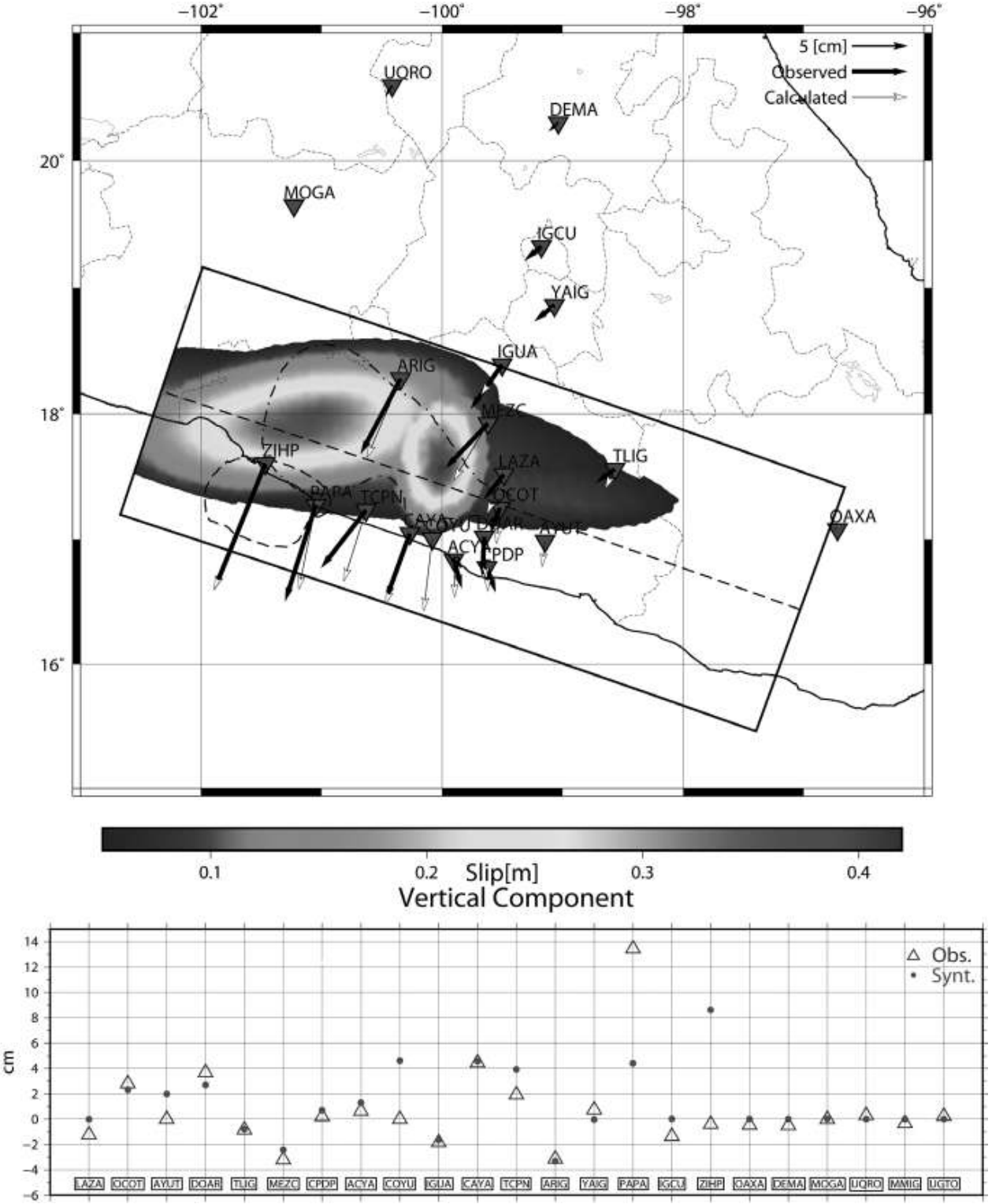
Figure 5 TOP: Slip distribution for the 2014 slow slip event. Dotted and dashed line is the isocontour from 12.5 cm from Radiguet et al., (2016). Dashed contour is the rupture area of the Papanoa earthquake. Three ellipses were necessary to fit data, one big ellipse and two small ones with the highest amplitudes. Thin and thick arrows are the calculated and observed displacements. Black arrows are the horizontal displacements. Red inverted triangles show GPS stations used. BOTTOM: Fits for the vertical component.
The second ellipse is down-dip of the Papanoa earthquake rupture area (dashed black polygon on Figure 5), near the limit between the seismogenic and transition zones. This patch could represent the afterslip of the Papanoa earthquake combined with the slow slip event; unfortunately, using only static displacements, it is not possible to separate the contribution of each one. Displacement at station TCPN shows a difference in direction with respect to PAPA and CAYA, which could be explained in part by the coseismic slip of the two aftershocks.
The third ellipse is the smallest one but the highest in amplitude and represents slip occurring down-dip of the Guerrero gap, within the transition zone at a depth of approximately 40 km, which confirms previous observations of slip in this region (Radiguet et al., 2012 and 2016 and the ones found in this work).
Following the April 18, 2014, Papanoa earthquake, two aftershocks with magnitudes 6.4 and 6.1 occurred within the Guerrero seismic gap where TCPN (Técpan de Galeana, Guerrero; Figure 5) station is located, and therefore their coseismic signature was recorded by at least this station. Because there is not enough information to retrieve the slip distributions for both earthquakes we cannot correct for this effect and the mismatch of TCPN displacement vector could be explained for this reason.
Observed and calculated displacements show good agreement. The difference in direction of the MEZC station could be explained by the afterslip of the Papanoa earthquake as well as the occurrence of the two aftershocks. In general, vertical displacements are difficult to fit. Nevertheless, results show good agreement with the vertical component for almost all stations. The largest misfits correspond to the stations closest to the rupture zone of the Papanoa earthquake (PAPA and ZIHP, Figure 5).
Discussion
The method has demonstrated to be efficient when following our proposed inversion strategy. This means that if the inversion leaves all parameters free, the solution found might not be physically representative, but if some a priori constraints are taken into account, the solution will have more validity. Several strategies were followed in order to find a more general approach. Starting with the inversion from one to five ellipses, with every new ellipse the misfit should change; lower misfit values do not necessarily mean that the model found is better than the previous one. For example, if the misfit for a two-ellipse model is lower than for a one-ellipse model could be due to the fact that the second ellipse is just trying to improve the misfit for one particular station instead of improving the overall misfit. This normally happens (for models of more than one ellipse) if the extra ellipse is isolated from the others.
The number of ellipses to invert could be one of the key steps in the process. First, it is recommended to invert one ellipse and keep adding more if the latter solution does not fit data equally good for all stations. Second, with every new ellipse, the previous solution should be fixed in order to let the new ellipse fit the rest of the data.
The initial model can be chosen as a random solution or by either the lower or upper bound of the parameter values. After hundreds of tries it was found that every initial model, evaluated with the same parameters (i.e. number of iterations, temperature, lower and upper bound parameters, etc), converges to a unique solution.
The best results for all events resulted when inverting for the first ellipse and find the best model, then fix that ellipse and invert for two ellipses leaving the second one free. Then invert for three ellipses keeping fixed the first two and so on. With this, the fit can progressively improve as a new ellipse is introduced. Also, the size and biggest amplitude of the ellipses should be restricted to at least half of the size of the fault plane and with every new ellipse the size restrictions should decrease (e.g., by half the size). Another strategy is to let one ellipse to be the biggest in area but with the lowest in amplitude and let the other ellipses to be smaller but with greater amplitudes.
Conclusions
A method to obtain a first approximation for the slip patterns of SSE was developed. The present implementation of the method considers a library of TF between the GPS stations operating in the Guerrero-Oaxaca region and each sub-fault. This library could be used for futures SSE and, if a new station is deployed in the region, then only that particular TF could be easily computed. Slow slip events have occurred every ~4 years at least since 1998 in the Guerrero region and it is reasonable to expect that another SSE may develop in ~2018.
The method was tested for three major slow slip events in the Guerrero region. For all the SSEs the method found models that fits data reasonably well even with the strong restrictions (geometry of the subducted plate and the shape of slip patterns). The low number of parameters to invert (18 for the three ellipse model) make the process fast enough to test different sets of parameters within a short time (all models were found within 10 min using an Intel Xeon CPU E5-2680 v2 @ 2.80GHz processor). Another important consequence of the low number of parameters is that it reduces the non-uniqueness, nevertheless, the best solution was found when a priori information was introduced. Locating the biggest observed displacements and restricting parameters related to the size and amplitude of the ellipses will improve the performance of the inversion process.
The number of ellipses does not seem to represent complexity of the event, but it contributes to finding a better fit, though this does not necessarily lead to a better model. Although more ellipses help to improve the fit we found that more than three will complicate the tectonic implications of the model. At least two ellipses were needed to fit data for the 2006 SSE model, while for the 2002 and 2014 three ellipses models were the best.
This method is thus a good approach to find slip patches within a plane at depth from surface static displacements. It reduces the number of parameters and is a simple good approach to be used in the Guerrero region of the Mexican Subduction Zone.

