


 nueva página del texto (beta)
 Inglés (pdf)
 Artículo en XML
 Referencias del artículo
 Enviar artículo por email
 Citado por SciELO
  Similares en
SciELO
Similares en
SciELO 
 Permalink
Introduction
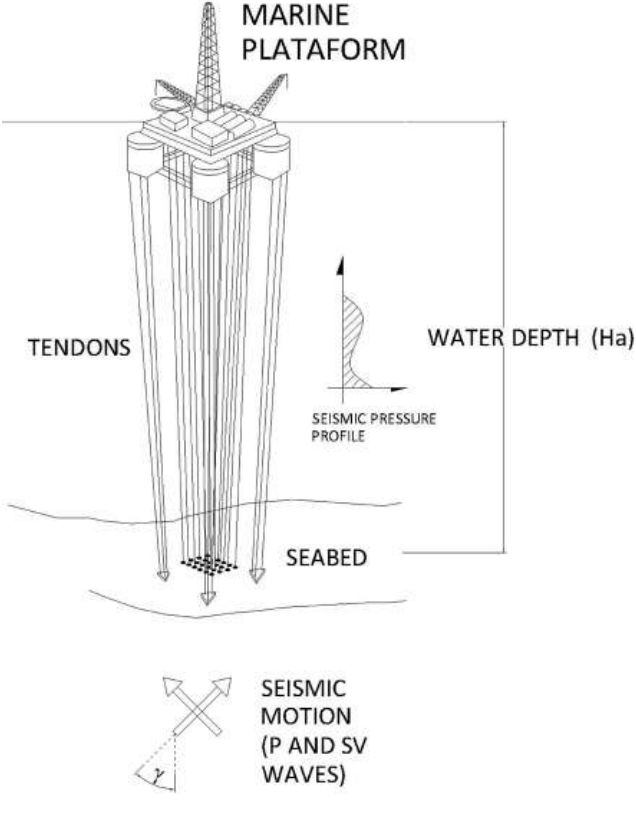
A large number of earthquakes have epicenters in offshore areas (Mangano et al,. 2011). Seaquakes are characterized by the propagation of vertical earthquake motion on the sea bottom as a compressional wave and cause damage to ships, and their effect on floating structures is a matter of great concern (Takamura et al., 2003). When the seabed is vibrating due to a seaquake, the compressional waves propagate with the water depth due to compressibility of water.
An analytical approach that can predict the dynamic response of a flexible circular floating island subjected to seaquakes was studied by Tanaka et al. (1991). The floating island was modeled as an elastic circular plate, and the anchor system to be composed of tension-legs. Linear potential flow theory applied to flexible floating island subjected to wind-waves and seaquakes was presented in Hamamoto et al. (1991), where the hydrodynamic pressure generated on the bottom surface of the island was obtained in closed form. The nonlinear transient response of floating platforms to seaquake-induced excitation was studied by Arockiasamy et al. (1983), where cavitation effects were considered.
A special boundary method for earthquake-induced hydrodynamic pressures on rigid axisymmetric offshore structures, including both the water compressibility and seabed flexibility, was presented by Avilés and Li (2001). A boundary integral equation was derived assuming that the seabed is a semi-infinite homogeneous elastic solid in order to analyze the seaquake-induced hydrodynamic pressu-re acting on the floating structure (Takamura et al., 2003). Boundary integral equations have been also used to calculate the hydrodynamic pressure caused by seaquake in layered media (Higo, 1997), and for three dimensional cases in Jang and Higo (2004). Recently, the boundary element method and the discrete wave number method have been used to determine pressures near the interface of fluid-solid models (Flores-Mendez et al., 2012, Rodríguez-Castellanos et al., 2011, 2014).
The Boundary Element Method (BEM) has been applied extensively to solve problems related to fluid-solid media subjected to seismic excitations. For instance, Schanz (2001) applied the BEM to study the dynamic responses of fluid-saturated semi-infinite porous continua subjected to transient excita-tions such as seismic waves. Moreover, irregular fluid-solid interfaces of oceanic regions or gulf areas under seismic wave propagation were analyzed in Qian and Yamanaka (2012), here important simulations of the water reverberation in the sea due to an explosive source were dealt, which show the applicability of the BEM to marine ambient. The dynamic response of a concrete gravity dam subject to ground motion and interacting with the water, foundation and bottom sediment was studied using the Boundary Element (Dominguez and Gallego, 1996). The model is able to represent continuous media with water, viscoelastic and fluid-filled pore-elastic zones. On the other hand, the dynamic response of liquid storage tank, including the hydrodynamic interactions, subjected to earthquake excitations was studied by the combinations of the boundary element and finite element methods (Hwang and Ting, 1989). Another application of BEM is focused on the seismic response of fluid-filled boreholes. In this way, in Tadeu et al. (2001), the BEM is used to evaluate the three-dimensional wave field caused by monopole sources in the vicinity of fluid-filled boreholes.
It is well known that Poisson´s ratio and Young´s modulus are sufficient parameters to linearly describe the stress-strain response under hysteretic conditions. In this work, a study of the sea water pressure profiles due to seismic actions of P- and SV-waves is presented. In fact, the ratio of P- to SV-wave velocities is a function of the Poisson´s ratio, only. Bowles (1988) and Wade (1996) classify the soils using its Poisson´s ratio. While, Sánchez-Sesma and Campillo (1991), Rodríguez-Castellanos et al. (2005) and recently Alielahi et al. (2015) used this criterion to characterize the soil where the wave propagation takes place. Hence, this criterion was followed as well.
This paper applies, for 2D problems in plane strain conditions, the Indirect Boundary Element Method to calculate the seismic pressure profile with the water depth due to the incidence of P- and SV- waves on the seabed (Figure 1), which is characterized by its soil properties. Wave amplifications are also highlighted. The formulation can be considered as a numerical implementation of the Huygens’ Principle in which the diffracted waves are constructed at the boundary from which they are radiated. Thus, mathematically, it is fully equivalent to the classical Somigliana’s representation theorem. The results are compared with those previously published. In the following paragraphs a brief explanation of the BEM applied to sea bottom subjected to seismic motions is given.
Formulation of the method
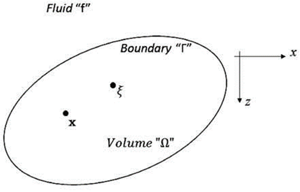
Consider the movement of an elastic solid, homogeneous and isotropic, of volumen delimited by its boundary (Figure 2), subjected to body forces b j (ξ, t) and null initial conditions. Introducing fictitious force densities ϕ i (ξ, t) in G, the fields of displacements and tractions could be written as Banerjee and Butterfield (1981):
where
For Eqs. (1), it is acceptable that these boundary integrals are valid for the main value of Cauchy. Then, if point x is allowed to approach to the boundary from inside of the region, at that time, Eqs. (1) are transformed to the next boundary equations:
were δ ij is Kronecker´s delta.
The problem was changed to the frequency domain, accepting that the incident waves have harmonic dependency with time, of type e iwt (i.e. u j (x, t)= u j (x, w)e iwt ), where w is the circular frequency and “i” is the imaginary unit. The displacements and tractions can be expressed as follow:
If the body is a fluid of volume Ωw delimited by its boundary Γw then the next functions represent the displacement and pressure fields:
where ψ(x, w) is the force density of fluid, ρ is the fluid density, G
f
(x, ξ, w) is the Green function for fluid pressure and is given by
The boundary conditions of the problem, according to Figure 1, are:
On the free water surface, the pressure is null, it means:
Onthe seabed:
Continuity of normal displacement:
Null shear in solid-water interface:
The tractions on the solid are balanced with water´s pressures
where ni is the unit normal vector associated to direction “i”,
If the boundary conditions, Eqs. (5)-(8) are expressed, using the integral representations, Eqs. (3) and (4), neglecting the body forces, and if the boundaries (Γ and Γ w ) are discretized in Nel boundary elements, then the following system, known as Fredholm´s system of integral equations of second kind and zero order is found.
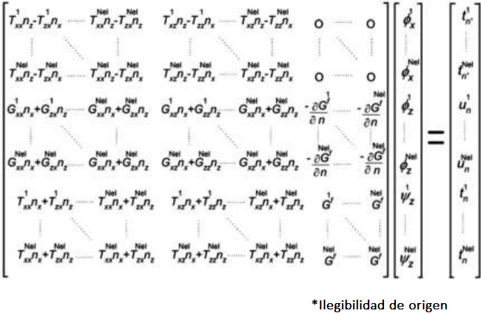
Once the solution of equation (9) is obtained, the displacement and pressure fields of equations (3) and (4), respectively, can be calculated. Additional details on the treatment to obtain the system of integral equations (9) can be consulted in Rodríguez-Castellanos et al. (2014).
Verification of the method and numerical examples
Verification
Wong (1982) and Kawase (1988) reported the seismic amplifications for the case of a topography with semicircular canyon shape of radius “a” (Figure 3d). They considered an elastic solid medium (with the properties shown in Table 1) in contact with an acoustic (vacuum) medium showing seismic amplifications in the solid surface between
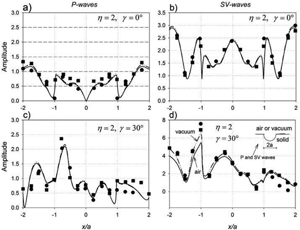
Figure 3. Comparison of results obtained by Wong (1982) (circles), Kawase (1988) (squares) and current formulation by BEM (lines). Solid line shows displacements in the x-direction for an air acoustic medium, while dash-dot-dot line shows displacements for a vacuum one.
Table 1. Elastic properties for elastic and acoustic media.
|
|
|
|
Observations | |
| Air Bedford and Drumheller (1994) | 330 | ----- | 1.29 | only for Verification |
| Elastic médium Wong (1982) and Kawase (1988) | 1998 | 1000 | 2500 | only for Verification |
In the present formulation, it is possible to consider that the high of the acoustic medium is approaching to infinity (H a ⟶∞) (and such properties are from the air (Table 1). H a is the water depth. Moreover, this method can deal with a solid-vacuum interface; the same problem studied by Wong (1982) and Kawase (1988) will be exactly resolved in the present study. The obtained results for the acoustic (air or vacuum) medium in contact with a solid one are displayed in Figures 3 and 4. The receivers are located on the seabed. Circles represent results by Wong and squares by Kawase. The present results are plotted with lines. In general, it is possible to appreciate a good match between the results found with the current formulation and those from the mentioned references, for both displacements and P- and SV-wave incidences.
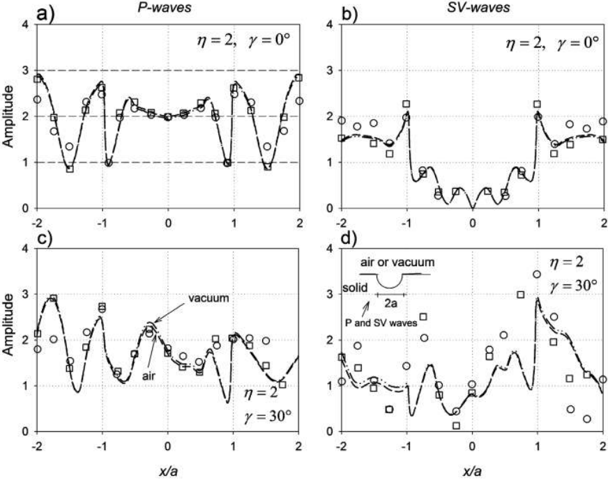
Figure 4. Comparison of results obtained by Wong (1982) (circles), Kawase (1988) (squares) and current formulation by BEM (lines). The striped line represents displacements in z-direction for an air acoustic medium, while dash-dot-dot line shows displacements for a vacuum one.
The use of the Green’s functions for infinite spaces, expressed in terms of Hankel’s functions of second kind, is an advantage of our integral formulation. Green’s functions for a half space can be also used in problems where a free surface is present. However, these functions are more complex than those for the infinite space and do not represent substantial save in computational requirements. On the other hand, we only modeled a finite part of the water and interface. Such truncation induces artificial perturbations caused by diffractions at the edges of the numerical model. However, these perturbations are characterized by small amplitudes and their reflections inside the model are negligible. The simplest solution is to choose a surface length large enough that the fictitious perturbations fall outside the observational space-time window. Then, edge effects due to the finite size of the discretized boundaries can be neglected; therefore, absorbing boundaries are not required.
The use of dimensionless frequencies has been usually employed to express the displacement fields of soil structures under seismic motions. In this context, several authors have used dimensionless frequencies to calculate strong ground motions or surface motions due to seismic movements. For instance, Trifunac (1973) (η=0.0 to 3.0), Wong (1982) (η=0.5,1.0,1.5,2.0), Sánchez-Sesma and Campillo (1991) (η=0.0 to 4.0), Rodríguez-Castellanos et al. (2005) (η=0.0 to 3.0) and recently Alielahi et al. (2015) (η=0.5, 1.0) used this criterion. In this work, results using η=0.0 to 4.0 are presented, this interval can be considered within the range of interest in earthquake engineering and seismology.
Numerical Examples
In order to develop numerical examples and show the influence that soil properties have on the propagation of compressional and shear waves that affect the sea bottom, and subsequently in pressure states with the water depth, the following elastic parameters were used for the analyses (see Table 2).
Table 2. Parameters used for analyses
| Elastic medium | SV-wave velocity (β) (m/sec) | Density (ρ) (kg/m3) | Poisson’s ratio (υ) | Reference |
| 1 | 3000 | 2100 | 0.25 | |
| 2 | 400 | 1700 | 0.35 | Huerta-Lopez et al. 2003 and 2005 |
| 3 | 190 | 1400 | 0.40 | |
| 4 | 90 | 1300 | 0.45 | |
| 5 | 20 | 1320 | 0.495 | Roever et al., 1959 |
The pressure profiles show many different behaviors that depend mainly on the soil properties
and the type of incident wave. For example, in Material 1, a lower amplification
of pressures due to P-wave incidence is obtained, compared with the
amplification obtained for Material 5 (see Figure
5). In Figure 5, the pressure
profiles for the non-dimensional frequency of
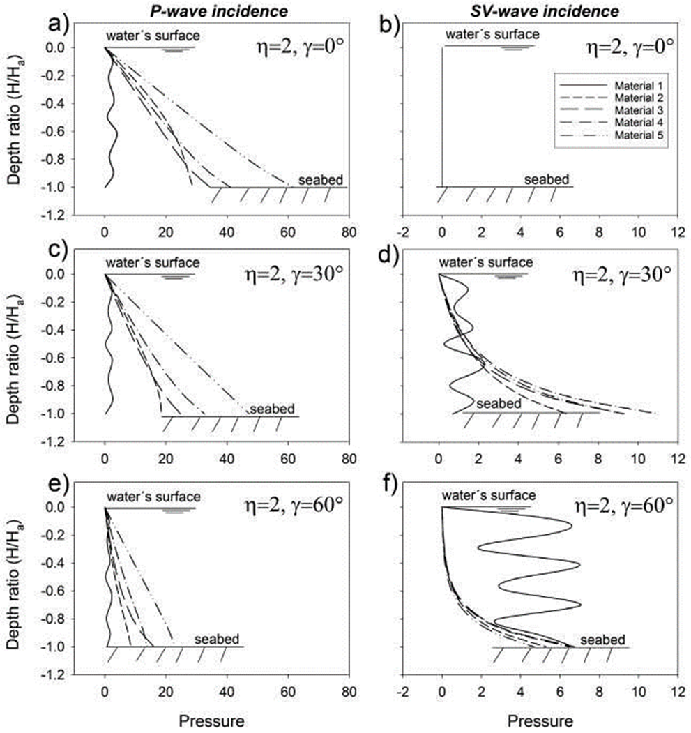
Figure 5. Pressure spectrum for different soil properties of seabed and incident angle of P- and SV-waves, for a flat bathymetry.
For Material 1, the underlying solid pressure variation with the water depth shows relatively small values for P-wave incidences with the three selected angles (0, 30 and 60 degrees) because of the impedance contrast between solid and fluid. On the other hand, for incoming SV-waves and large incidence angle (60 degrees) the horizontal phase velocity is quite large, as compared with the propagation velocity within the fluid. This and the polarization of motion induce significant emission of waves within the solid for a quasi- vertical direction.
Figure 6 depicts the behavior of pressures when P- and SV-waves impact a sinusoidal bathymetry (see detail in Figure 6f). The material properties and incident angles of the elastic waves are the same as in Figure 5. For the case of P-waves, the pressure field shows small variations in comparison with a flat interface. However, for the case of SV-waves, diffracted pressure waves are present for an incident angle γ=0º. For angles of γ=30º and γ=60º the pressures describe patterns similar to those for a flat interface (Figure 5), but they reach lower values.
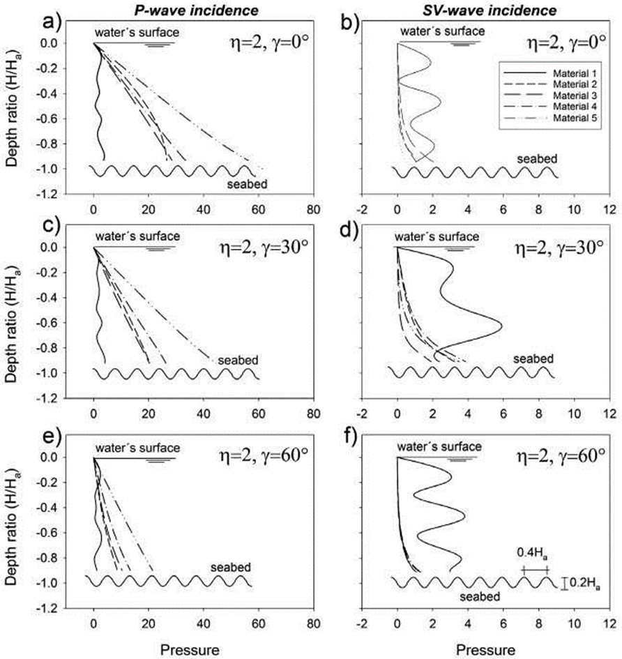
Figure 6. Pressure spectrum for different soil properties of seabed and incident angle of P- and SV-waves, for a sinusoidal bathymetry.
Figure 7 shows the pressure fields obtained at several water depths. These pressures were calculated at six locations (H/Ha =0, -0.20, -0.40, -0.60, -0.80 and -1.0) for a frequency range of 0<η<4.0. The soil has the properties of Material 1, according to Table 2. In this case, normal (γ=0°) and oblique (γ=30°) P- and SV-wave incidences on a flat interface (Figure 7a) are considered. It must be emphasized that for all the cases null pressures are obtained on the water surface (Figures 7 b-e), as expected. On the other hand, null pressures are obtained, when an SV-wave impacts with an angle γ=30° (Figures 7 c, g, k, o, s, and w). It can also be said that several peaks are present in the graphs, which are associated with the resonances generated by waves interacting between the water surface and the seafloor. These peaks appear clearly in the case of normal P-wave incidence and near to the seafloor (H/Ha = -1.0, Figure 7v). In addition, it is noticeable that the oblique P- and SV-wave incidences (γ= 30°) generate pressure fields at the six mentioned locations. However, these pressures show less amplitude than those generated by a normal P-wave incidence. In general terms, the greatest pressures are present in the proximity of the seafloor (Figures 7v, x and z), which have been also highlighted in the previous analyzes.
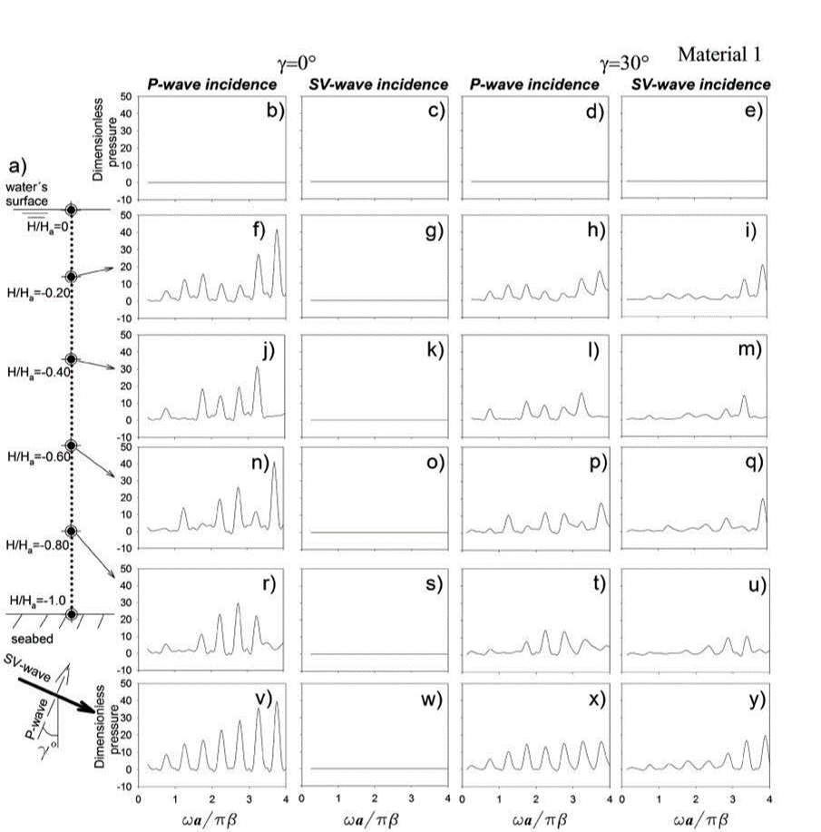
Figure 7. Pressure spectrum at several water depths. The range of dimensionless frequency is 0<h<4.0.
Figure 8 displays the propagation of P-waves calculated in 51 receivers spaced 0.04 H/H a . The propagation is presented for five types of seabed, according to Table 2, for Materials 1 to The first 25 receivers are located in the solid, see bottom figures showing displacements in the z-direction. Displacements for the x-direction are zero when a normal P-wave impacts the interface. The last 26 receivers are located in the water, see top figures showing the pressure generated by the incidence of P-waves. A normal incidence (γ=0°) of P-waves that impinges on a flat and horizontal surface does not create diffraction in the x-direction. In general terms, an incident wave that is propagating in the solid is transmitted to the fluid generating a pressure field. It can also be seen that the water surface causes the reflection of waves that propagate in the opposite direction. Later, in Figure 10 pressures obtained nearby seabed are discussed.
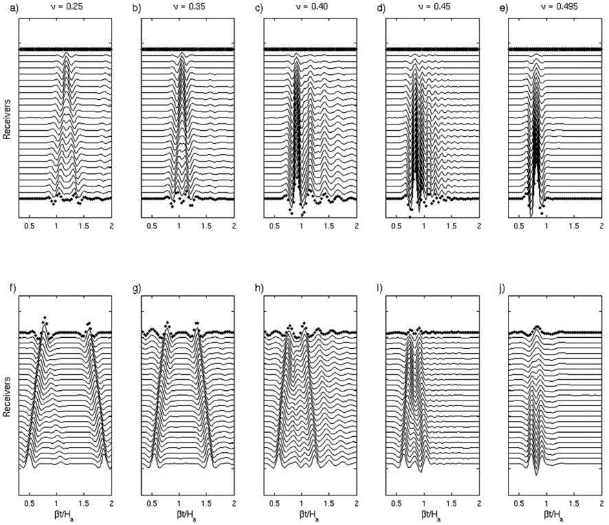
Figure 8 Propagation of compressional waves recorded at 51 receivers for different materials: wáter pressure (top figures) and displacement in z-direction in the solid (bottom figures).
In Figure 8, the displacements for 64 frequencies up to 15.39 Hz at the mentioned receivers were computed in the frequency domain. In order to simulate the motion with the time we used the FFT algorithm to calculate synthetic seismograms using a Ricker wavelet. This pulse has a temporal dependence given by:
where
t p = characteristic period, and t s = time-lag or offset. In the present computations t p = 0.259 sec and t s = 0.779 sec were used. The time scale is given by β t /H a (normalized time).
Physically, η represents the ratio of the water depth (Ha) to the incident wavelength. The range of frequency (64 frequencies up to 15.39 Hz) permits to generate a Ricker pulse with a wavelength that can “feel” the interface and the water surface. According to this, Figure 8 makes clear that several wave diffractions and reflections take place in the water, for the selected wavelength.
In Figure 8, the incidence of elastic waves on the interface produces the phenomenon of reflection and refraction of waves and also the appearance of interface waves (Scholte waves). This last type of wave appears once the interface is excited. The energy that carries this wave dissipates during its travel, radiating energy towards the fluid and the solid medium. In Figures 8a-j, the interface waves continue to radiate energy and generate variations in pressure after the first reflections and refractions have taken place. These pressure variations can be seen from 1.7 to 2 seconds for the case of Figure 8a, from 1.5 to 1.7 seconds in Figure 8b, from 1.3 to 1.8 seconds in Figure 8c and from 1 to 1.5 seconds in Figure 8d. In all these cases, the influence of the Poisson ratio on the pressure state in the fluid can be observed. A detailed study of the interface waves and their effect on pressure can be found in Borejko (2006).
The incidence of P- and SV-waves on the seabed could cause displacements in x and z-directions. The calculated amplitudes are dependent on the type of the seabed material and the incident angle of the seismic movements. Figure 9 shows the displacements produced in the seabed at frequency η=2 for incident P- and SV-waves at angles=0º, 30° and 60°. Materials 1 to 5 were analyzed. In general terms, the normal incidence of P-waves causes amplitudes of vertical displacement (z) close to 3 (Figure 9c). For other angles of in-cidence the displacement is lower. The normal incidence of SV-waves gives zero displacements in the vertical direction (Figure 9d), while for other angles of incidence such displacements are small compared to those caused by P-waves. The maximum displacement in the x-direction is produced by the normal incidence of SV-waves, these displacements decrease as the incidence angle increases. The diffraction caused by P-waves is very small for the incidences and 30°, whereas for γ=60º it reaches a value near to 2 for Material 1.
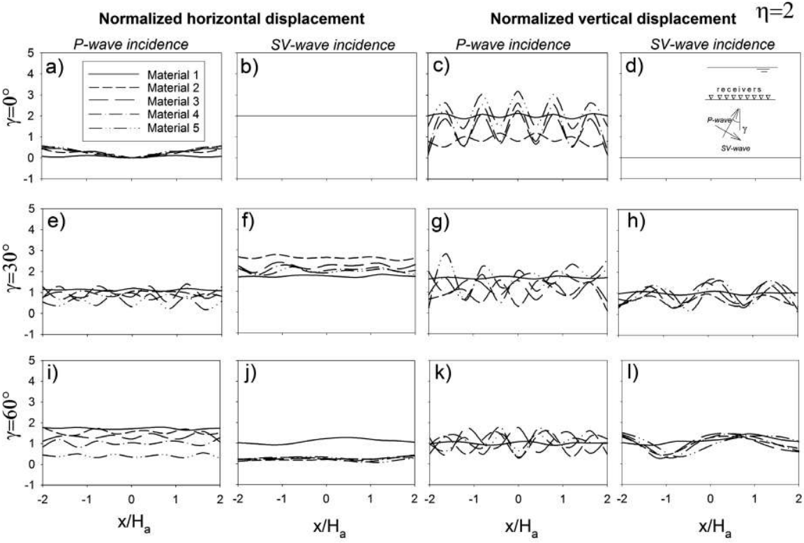
Figure 9. Displacement amplitudes calculated on seabed resulting from incidence of P- and SV-waves with angles of γ=0°, 30° and 60°.
Figure 10 presents the pressures in time domain, obtained in the vicinity of the seabed for Materials 1 to 5 and for normal incidence of P-waves. It is clear that for Material 5 strong amplifications in the range of 6.05 times are obtained in comparison with Material 1 (see Figure 10e). This result shows the importance of adequately characterizing the type of soil where marine structures will be located since strong amplifications of seaquakes can be present.
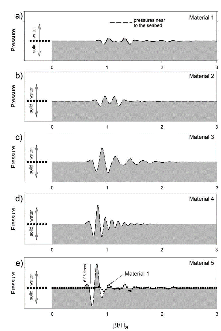
Figure 10. Maximum pressures calculated nearby the seabed for Materials 1 to 5, for normal incidence of P- waves.
Now, results for a layered medium are displayed. This medium is composed of an elastic half space (Material 1), a layer (Material 2)and the sea water. The elastic properties of the solid medium can be found in Table 2. The studied model is detailed on Figure 11e, where the localization of receivers 1 and 2 are also shown. Receiver 1 is located on the seafloor and receiver 2 is between the two solid materials. We studied two layer thicknesses, one of h/Ha =0.025 (Figures 11c and d) and another of h/Ha =0.05 (Figures 11a and b). These figures show the calculated seismic amplifications in such receivers for a frequency range 0< η<4.0. For this purpose, the normal incidence (γ=0°) of P- and SV-waves on the stratified medium (Figure 11e) is considered. In this figure, it is remarkable that the greatest seismic amplifications are obtained at Receiver 1, reaching a value of 15.57 for the incidence of P-waves (Figure 11a) and 18.36 (Figure 11b) for SV-waves. These values correspond to the case of a layer thickness of h/Ha =0.05. In fact, in this case, the layer with greater thickness generates larger seismic amplifications with respect to the layer of reduced thickness. In the case of h/Ha =0.025, the maximum amplifications obtained correspond to 11.08 (Figure 11c) for the incidence of P-waves and 16.25 (Figure 11d) for SV-waves. In addition, the presence of the layer causes more oscillations in the response associated with the P- waves, in comparison to the SV-waves. Such interactions generate sharp peaks in the response obtained. It should be noted that in all cases, the displacements calculated for the receiver 2 had an average value of 2. Strong amplifications by soft layer have been previously reported in the field of earthquake engineering and seismology. For example, one of the first contributions on seismic amplifications is that of Trifunac (1971), where he showed amplifications around 20 times the incident wave, for the case of an SH-wave hitting an alluvial valley. It should be mentioned that the normal incidence of P- and SV-waves does not cause displacements in the horizontal and vertical direction, respectively. It is important to emphasize that the presence of a soft layer can generate large seismic amplifications, which must be taken into account in the design of marine installations.
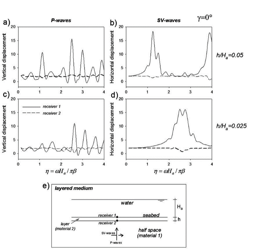
Figure 11. Vertical and horizontal amplifications due to the normal incidence of P- and SV-waves on a layered medium. The range of dimensionless frequency is 0<h<4.0.
In the case of an oblique incidence of elastic waves (P and SV), seismic amplifications are present for both components of displacement. Such amplifications can reach considerable values. Then, considering the models and materials of Figure 11, and hitting the médium with an incident angle of elastic waves of γ=30º, the seismic amplifications reach large values. For example, Figure 12c exhibits an amplification of 15.68 (at a frequency of η=3.62), which corresponds to the case of h/Ha =0.025 under the incidence of P-waves. On the other hand, the incidence of SV-waves generates amplifications of 15.11 (Figure 12h), which also corresponds to the case of h/Ha =0.025. This figure makes it clear that the oblique incidence of elastic waves can generate high seismic amplifications, for both components of displacement, although these amplifications are smaller than those obtained in the case of the normal incidence (γ=30º, Figure 11). It should be noted that Receiver 1 is again the one that reaches the largest seismic magnifications.
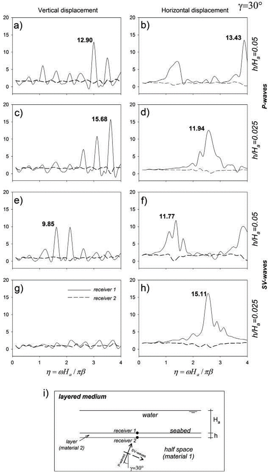
Figure 12. Vertical and horizontal amplifications due to the oblique incidence of P- and SV-waves on a layered medium. The range of dimensionless frequency is 0<η<4.0.
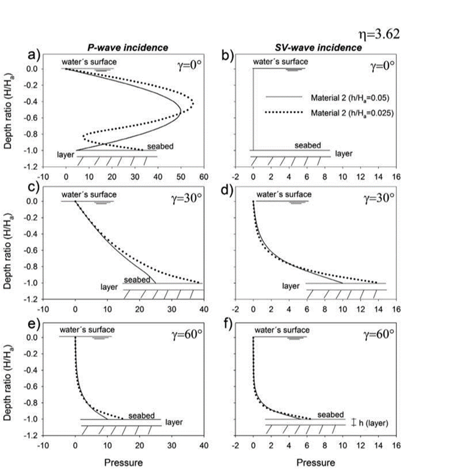
Finally, with the purpose of illustrating the effect that the presence of a layer has on the pressure field in the water, Figure 13 is included. Again, the models and materials used for the previous simulations were considered. But now the frequency of η=3.62 has been selected, which corresponds to the frequency where the greater amplification for previous case was obtained (Figure 12c). To display the pressure field in the water, three incident angles of elastic waves (γ=0º, 30° and 60°) were selected. The layer is formed by Material 2 and its thickness is given by h/Ha =0.025 and 0.05. The pressure field for the thinner layer is graphed with a dotted line, while for the thick layer a continuous line is used (Figure 13b). It should be noted that the presence of the layer causes variations in the pressures calculated throughout the water depth and mainly in the proximity of the sea bottom. It is important to emphasize that for these cases and for the frequency studied (η=3.62) greater pressures are achieved for the case of h/Ha =0.025. This result is more evident for the incidence of P-and SV-waves with an incident angle of γ=30º (Figures 13c and d). On the other hand, the incidence of SV-waves with γ =0º does not generate pressure fields in the water (Figure 13b). For the incidence of elastic waves with an angle of γ=60º, the pressure field practically remains unchanged, for both layer thicknesses.
Conclusions
This paper applies the Indirect Boundary Element Method to calculate the seismic pressure profile with the water depth due to the incidence of P- and SV-waves on the seabed. Two dimensional problems, in plane strain conditions, are considered. This formulation can be considered as a numerical implementation of the Huygens’ Principle in which the diffracted waves are constructed at the boundary from which they are radiated. Thus, mathematically it is fully equivalent to the classical Somigliana’s representation theorem. The results suggest that the pressure profile shows very different behaviors that depend mainly on the soil properties and the type of incident wave. Overall, the incidence of SV-waves produces a less pressure magnitude than that obtained for P-waves. In most cases studied, the maximum pressure obtained is located nearby the seabed. This is important for the design of facilities supported on the seabed. Moreover, it has been shown that for a soil type of Material 5, seismic amplifications on the seabed are 6.05 times larger than those obtained for Material 1. Furthermore, results from the layered numerical model evidence that large seismic amplifications may be found, reaching values up to 15.57 and 18.36 times the incident P-and SV-wave, respectively. These results demonstrate the importance of adequately characterizing the type of soil where marine structures will be located.

