Introduction

Groundwater modeling as a tool for sustainable development and utilization of groundwater resources in land subsidence studies requires knowledge of the hydrogeologic properties of the medium. A number of studies have shown that parameters such as hydraulic conductivity and porosity of porous media exhibit spatial variations. Most of the times, these variabilities can only be determined at few and sparse locations. Thus, there is uncertainty in the characterization of the spatial variability of those properties. Owing to this uncertainty, predictions conducted with groundwater flow models are also uncertain. To make plausible predictions and reduce the associated uncertainty, stochastic inverse modeling techniques are frequently applied. These techniques allow the identification of parameters and the quantification of parameter and prediction uncertainty consistent with the measured data and the groundwater flow model.

In subsurface hydrology, hydraulic conductivity fields are often characterized assuming that its spatial variability can be interpreted as a realization of a random field model ^{(Dagan, 1989}; ^{Gelhar, 1993)}. The parameterization of the random field is obtained through the observations of the realization itself assuming the field is ergodic ^{(Deutsch and Journel, 1992}; ^{Chilés and Delfiner, 1999)}. Then, inferences at unobserved locations and the uncertainty of these inferences are determined on the basis of the direct observations by either estimation or simulation techniques (e.g. ^{Journel and Huijbregts, 1978}; ^{Chilés and Delfiner, 1999)}. While estimation techniques provide one single “best” estimate of the hydraulic conductivity field, simulation techniques yield multiple realizations of that field ^{(Journel and Huijbregts, 1978)}. In order to reduce the uncertainty in the inference of the hydraulic conductivity field, indirect observations of it, e.g., of hydraulic heads, are also taken into account in these tasks by solving the typical inverse problem of hydrogeology ^{(Chilés and Delfiner, 1999)}. Other informative variables such as flow rates and species concentrations may also be incorporated in the inference process to further constrain the spatial fluctuations of the conductivities. Although solutions to the inverse problem lead to hydraulic conductivity fields which are compatible with the measured hydraulic head data, it is recognized that there are an infinite number of other conductivity fields which may also match the same hydraulic head data ^{(RamaRao et al., 1995)}. The inverse problema is therefore ill-posed and a unique, exact solution is generally not available. Instead, a solution which coincides with the observations is commonly sought ^{(Tarantola, 2005)}.

The inverse problem can be solved under steady conditions or under transient conditions using estimation or simulation techniques ^{(Gómez-Hernández and Wen, 1994}; ^{Chilés and Delfiner, 1999)}. A comprehensive review of the evolution of several methods for solving the stochastic inverse problem in hydrogeology has been presented elsewhere ^{(Zhou et al. 2014)}. Among these approaches, simulation-based inversion techniques are often preferred over estimation-based inversion techniques because it has been proven that the single “best” estimate provided by the latter does not capture the range of variability of real fields of conductivities. As a result, flow and transport predictions conducted in these fields are very poor ^{(Gómez-Hernández and Wen, 1994)}. The most widely accepted simulation-based inversion techniques in groundwater modeling use the Monte Carlo (MC) method. Within the MC framework, the available observations of the state variables are integrated into a prior random field of conductivities through an iterative procedure to obtain a posterior random field of conductivities expressed as a set of conditional simulations. Examples of such kinds of approaches are: the self-calibration method ^{(Sahuquillo et al., 1992}; ^{Gómez-Hernández et al., 1997)}, the pilot-point method ^{(RamaRao et al., 1995)}, the Markov-Chain MC method ^{(Oliver et al., 1997)}, the gradual deformation method ^{(Hu, 2000}; ^{Capilla and Llopis-Albert, 2009}; ^{Hu et al., 2013)} and the random mixing method ^{(Bárdossy and Hörning, 2016)}. One common characteristic to all of these MC-based inversion methods is that they are formulated as optimization problems where the unknown parameter field is represented by the nodes of a mesh. Thus, the use of dimensional reduction techniques is indispensable in large dimensional problems. The main difference among the approaches is the way the optimization problem is solved.

An alternative MC-based inversion technique that can be used to integrate available observations of the hydraulic head into a prior random field model of conductivities is the Ensemble Kalman Filter (EnKF). In this approach, the observations are integrated sequentially in time using the groundwater model itself to evolve the hydraulic head field in a physically plausible manner ^{(Katzfuss et al., 2016)}. The EnKF was developed by ^{Evensen (1994)} as an extension of the Kalman Filter (KF) ^{(Kalman, 1960)} to deal with non-linear systems. The main difference between EnKF and KF is that the former uses an ensemble representation for the state variables from which any statistical moment can be calculated whenever it is needed. Instead of using the MC method, earlier extensions of the KF used perturbation theory to handle non-linear dynamics. This is the case of the Extended KF (EKF) ^{(Evensen, 1992}; ^{Leng and Yeh, 2003)}. However, it has been found that the EnKF outperformed the EKF, especially in highly non-linear systems ^{(Miller et al., 1999}; ^{Reichle et al., 2002)}. The EnKF differs from other MC-based filters, such as particle filters, in the process by which the observations are integrated into the prior random field model.

The EnKF procedure consists of two main steps. The first is the forecast step, which uses MC sampling to propagate the uncertainty in the hydraulic conductivity field through the groundwater model to approximate the spatiotemporal evolution of the hydraulic head field at the time the observations are available. The second is the update step that integrates the measured hydraulic head data into the prior random field model of conductivities by conditioning each prior realization to the available observations. The conditioning process is performed only on the basis of the available data at the time of analysis using a linear estimation technique. Thus, only the mean, auto-covariance and cross-covariance functions are used when computing the posterior random field of conductivities. This strategy lends the scheme computational efficiency and makes it suitable for large dimensional problems, yet the forecast step may still be highly demanding in terms of computation. Since the conditional simulations thus obtained are consistent with the system dynamics, predictions of response variables and an investigation of the uncertainty of these predictions can also be conducted simultaneously.

The EnKF only converges to an optimal solution when the random fields involved are multi-Gaussian and when the functional relationship between state and parameter variables is linear. Due to the non-linearity of the groundwater equations, it seems reasonable to expect that state fields will be non multi-Gaussian even in multi-Gaussian parameter fields. Thus, assuming joint multi-Gaussian distributions between conductivities and heads is often not correct in practice. Moreover, in multi-Gaussian random fields the spatial correlation structure is symmetric; i.e., the values at opposite percentiles with respect to the mean present exactly the same spatial correlation structure ^{(Journel and Deutsch, 1993}; ^{Journel and Zhang, 2006)}. The highest continuity is observed at mean values and the extreme high/low values appear as isolated clusters. As a result, connected paths of extreme values do not occur in multi-Gaussian random fields ^{(Gómez-Hernández and Wen, 1998}; ^{Knudby and Carrera, 2005)}. On the contrary, field evidence suggests that the patterns of spatial variability in natural soil formations differ significantly from such multi-Gaussian dependence characteristics. ^{Journel and Alabert (1989)} found stronger spatial correlation structures at low values than at high values in field measurements of air permeability taken on a vertical slab of Berea sandstone; this stronger correlation was even stronger than that imposed by a multi-Gaussian random field model. Asymmetric correlation structures have also been found in conductivity fields with relatively small heterogeneity ^{(Haslauer et al., 2012)}. Thus, natural porous media seem to be non multi-Gaussian with respect to their spatial distribution of conductivities independently of their degree of heterogeneity.

Several extensions of the EnKF have been examined in the last decade in order to achieve a more versatile tool capable of handling non multi-Gaussian random field models in parameter identification problems. ^{Sun et al. (2009)} reformulated the update step of the EnKF using Gaussian mixture models and clustering techniques. ^{Sarma and Chen (2009)} developed a generalization of the EnKF based on kernel principal component analysis. ^{Emerick (2017)} presented an investigation of the performance of different principal component analysis-based approaches. ^{Bertino et al. (2003)} modified the update step of the EnKF by applying Gaussian transformations. The advantages of this last extension compared to the classical EnKF method were confirmed in several studies ^{(Zhou et al. 2011}; ^{Li et al. 2012}; ^{Schöniger et al. 2012}; ^{Erdal et al. 2015)}. One common characteristic to all of these EnKF-based methods is the use of auto-covariance and cross-covariance functions as unique descriptors of the spatial dependence at each update step. Unlike these approaches, ^{Zhou et al. (2012)} developed the so-called Ensemble PATtern matching method (EnPAT) based on multiple-point geostatistical simulation techniques which use multiple-point covariance functions rather than traditional two-point covariance functions to determine the spatial correlations. Extensions of this approach were developed later ^{(Li et al. 2013}, ²⁰¹⁴, ²⁰¹⁵⁾. Although the EnPAT method outperforms the classical EnKF and eliminates the multi-Gaussian assumption implicit in the update step of the latter ^{(Li et al. 2015)}, it strongly relies on the concept of training image; i.e. a conceptual model of the geological structure of the formation under study, the construction of which can be problematic, especially in 3D applications, and the benefit of which is more evident in fluvial deposits than in other type of geologic formations.

The EnKF with Gaussian transformations (tEnKF) has been particularly well accepted in several geophysical areas ^{(Bertino et al. 2003}; ^{Simon and Bertino, 2009}, ²⁰¹²; ^{Béal et al. 2010}; ^{Zhou et al. 2011}; ^{Li et al. 2012}; ^{Schöniger et al. 2012}; ^{Xu et al. 2013}; ^{Erdal et al. 2015}; ^{Zovi et al. 2017)}. In subsurface hydrology, it has been applied to the identification of the hydraulic conductivity of synthetically generated channelized aquifers that display the same asymmetry as the prior random field model ^{(Zhou et al. 2011}; ^{Li et al. 2012}; ^{Xu et al. 2013)}. Thus, the domain under study has the same spatial variability characteristics as those of the set where the spatiotemporal evolution of the hydraulic head field is sought. As a result, the performance of tEnKF is promising because the deviations from the reference field are then corrected, up to a certain extent, with the update steps. However, these studies do not take into account the risk of introducing a systematic bias in the spatiotemporal evolution of the hydraulic head field during the forecast steps that the update steps may not correct over time. While they attribute the promising performance of tEnKF to Gaussian transformations, they disregard the implications of the information incorporated in the prior conductivity fields. This information should be taken into account to explain the performance of the tEnKF because the update step remains suboptimal and is performed under the multi-Gausian model which is unable to capture channelized structures with the covariance function as the sole descriptor of an evolving spatial dependence. The absence of knowledge about higher order moments of the parameter field inevitably implies a risk of introducing such systematic bias.

This paper proposes that in order to evaluate the performance of tEnKFs, applications in synthetically generated random porous media should take into account the risk of systematic bias by incorporating prior knowledge with a multi-Gaussian conductivity correlation structure, and by considering the spatial distribution of the hydraulic conductivity of a reference field as having an asymmetric correlation structure. This view of the problem follows the idea of ^{Kerrou et al. (2008)}, yet differs significantly from its mathematical framework and scope. Our experimental setting is closer to a common situation found in practice where one has access to a rough approximation to the mean, variance and auto-covariance function of the real field, but the asymmetry of the spatial correlation structure of that field is unknown. As an example of this application, this paper identifies hydraulic conductivities using the tEnKF by solving a one-dimensional, single phase flow problem in a continuous random porous medium. To explain the hypothesis underlying both EnKF and tEnKF and to establish a clear link between the tEnKF and the stochastic simulation of conditional random fields, common concepts in Geostatistics are used. Ultimately, the aim of this paper is to motivate further discussions about the benefit of incorporating transient hydraulic head responses in the identification of hydraulic conductivity fields subject to this kind of constraint and about further potential improvements to the update step of the EnKF to overcome the multi-Gaussian assumption.

Groundwater flow equations

In this section, the dynamic model describing single-phase fluid flow in a one-dimensional, vertical, fully saturated porous medium with spatially variable hydraulic conductivity is analyzed:

subject to initial and boundary conditions

where H is the hydraulic head [L] in the domain Ω, x is the spatial coordinate (x = x ₃ [L], where x₃ represents the vertical coordinate which is positive upward), K _S (x) is the saturated hydraulic conductivity [L/T], S _S is the specific storage [L^-1], h ₀ represents the initial head and h ₁ the prescribed head at Dirichlet boundary Γ _D.

In the present example, specific storage as well as initial and boundary conditions are treated as deterministic constants. An error-free dynamic model is also assumed. Hence, the model prediction is only affected by the un-certainty in K _S (x). To model this uncertainty, a stationary random field model is adopted. In such an approach, Y(x) defines the collection of n continuous scalar random variables of the natural logarithm of the saturated hydraulic conductivity, i.e. Y(x) = ln(Y _S (x)) indexed at the spatial locations x in the domain W _x with W _c ∈ 𝕽¹. Since K _S (x) is a random field, Equation (1) becomes a stochastic differential equation and the flow response H becomes a spatiotemporal random field. K _S (X, t) is defined as the collection of N continuous scalar random variables of the hydraulic head indexed at the spatial locations c in the domain Ω _x with Ω _x ∈ 𝕽¹ and times t∈{0, 1, 2,...}. Although Y(x) is assumed as stationary, H(X, t) will be non-stationary in space and time because the domain is bounded ^{(Zhang, 2002)}. In the following formulations, an ensemble interpretation of both random fields is applied.

The EnKF method

In this section, an alternative formulation for parameter estimation of the EnKF based on common concepts in Geostatistics is presented.

The EnKF method with transformed data (tEnKF)

There are two additional steps and one modified update step that have to be implemented in the EnKF method with transformed data (tEnKF). These three steps are described in this section using common concepts in Geostatistics. Then, some useful formulas for post-processing the results and recommendations for the numerical implementation of the tEnKF are presented.

Gaussian transformation step

Under the multi-Gaussian hypothesis implicit in the classical EnKF procedure, the univariate conditional CDF of Y(x), given that N_h observations of H(X₁, t=1) are known, will be Gaussian with conditional expectation and conditional variance given by the simple Kriging (cokriging) estimates ^{(Journel and Huijbregts, 1978)}. However, for the Kriging variance to be an unbiased estimate, both Y(x) and H(X₁, t=1) have to be zero-mean Gaussian random fields ^{(Shinozuka and Zhang, 1996)}. ^{Bertino et al. (2003)} realized this situation and therefore proposed to apply Gaussian transformations, at least locally, to both random fields. The Gaussian transformation maps non-Gaussian distributed random variables into Gaussian random variables (with zero mean and unity variance) according to:

Y~xi=Φ-1(FY(y;xi)) (6)

H~xi, t=1=Φ-1(FH(h;xi;t=1)) (7)

where Φ^-1(⋅) is the inverse of the univariate Gaussian distribution function, and F_Y (y; x _i ) and F_H (h; x _i ; t=1) are the local distribution functions of Y(x) and H(X₁, t=1), respectively. In the tEnKF the empirical versions of these distribution functions are used. The empirical distribution function is defined by Fnc=1/nr∑j=1nrIcj≤c, where I{•} stands for an indicator random variable that takes a value equal to 1 whenever its argument is true, and 0 otherwise with n_r equal to the number of log-conductivity fields. It should be recalled that the empirical distribution function will converge to its theoretical counterpart as the number of realizations in the ensemble tends to infinity ^{(Billingsley, 1995)}. The variables with the tilde in Equations 6-7 symbolize the transformed random variables. In addition to the transformations expressed by these equations, a standardization of the observations at each location have to be applied. The function relating y to y or h to h in the x-y Cartesian plane, is called the Gaussian anamorphosis function and was introduced by ^{Rosenblatt (1952)} (Figure 1).

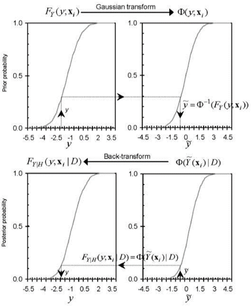
Figure 1. Transformation step of the EnKF method: a) Gaussian transformation process, b) Back-transformation process. 

Note that since only marginal transformations are applied, the joint multivariate distributions of Y(x) and H(X₁ , t=1), as well as the multivariate distributions of H(X₁ , t=1) and Y(x), are not modified.

Numerical implementation

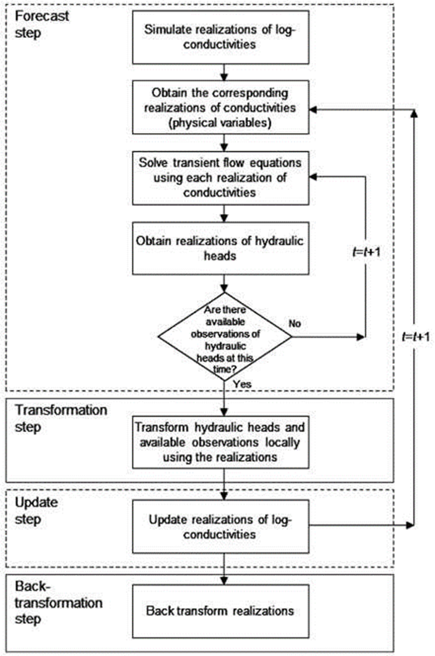
The mathematical model described in the previous sections is coded in FORTRAN programming language on the LINUX platform and run in the HPC cluster “Tonatiuh” at the Institute of Engineering, UNAM. A block diagram describing its numerical implementation is depicted in Figure 2. Note that the conditioning process is repeated at the next time at which observations are available, but the new prior log-conductivity random field becomes the posterior one at time t=1.

Figure 2. Block diagram of the EnKF with transformed data (tEnKF). 

Application of the tEnKF to the identification of conductivities

Multivariate spatiotemporal random fields have been used in a variety of geophysical applications. For example, ^{Bodas-Salcedo et al. (2003)} combined spatiotemporal random fields with the Kalman filter method to predict solar radiation in the earth-atmosphere system; ^{Suciu (2014)} used a diffusion model to predict solutes transport in groundwater under uncertainty about spatiotemporal evolution of velocity fields; a similar approach was used by ^{Suciu et al . (2016)} to model reactive transport; ^{Sanchez et al . (2016)} developed a spatiotemporal dynamic model based on the classical EnKF for Bayesian inference of rainfall; and ^{Liang et al. (2016)} used a stochastic groundwater flow model to analyze the effect of uncertainty in recharge and transmissivity on the spatiotemporal variations of groundwater level in an unconfined aquifer. Finally, ^{Moslehi and de Barros (2017)} investigated the impact of uncertainty in spatial variability of soil hydraulic conductivity on several environmental performance metrics that are relevant for environmental risk assessments, such as species concentrations and arrival times, using a stochastic advection-dispersion model to represent the spatiotemporal evolution of the concentration field.

In this paper, the tEnKF is applied to infer the hydraulic conductivity field in a confined porous medium on the basis of the observed spatiotemporal variations of the hydraulic head field. For the sake of simplicity, groundwater flow through a one-dimensional, vertical, fully saturated random porous medium is considered (Equations 1-2). It is assumed that hydraulic head at the lower boundary of the porous medium diminishes at a constant rate known from historical records and that this decrement is associated with groundwater withdrawal from wells located farther away. This simplified setting allows useful preliminary evaluations of the tEnKF. However, it is recognized that these two hypotheses can be avoided by 3D modeling of the system including the wells, and by considering that the spatial variability of the hydraulic conductivity in porous media is in fact 3D. The coupling of this dynamic model within the tEnKF is being developed and the results will be presented in further publications.

The porous medium is 40m deep and is discretized into 80 finite elements each with a length of 0.5m. Each finite element e_i for i=1,…,80 is assigned a log-conductivity value y^ref (x _i ) according to the following procedure. First, a multi-Gaussian field g(x) with exponential auto-covariance function and correlation scale a=2.5m is simulated using a modified version of the SGSIM random field generator ^{(Deutsch and Journel, 1992)} (Figure 3a). Second, the V-transform is applied in the following manner ^{(Bárdossy and Li, 2008)}:

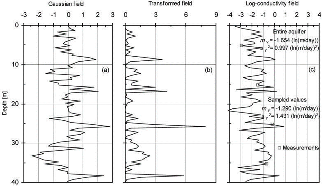
Figure 3. One dimensional fields: a) Initial Gaussian field, b) Field after applying the V-transform with parameters m=0 and k=1 to the initial Gaussian field, c) Final log-conductivity field after imposing a marginal normal distribution with expected value m_Y=-1.654 and variance s_Y²=0.997 to the V-transformed field. Statistics of sampled values (empty squares) are also reported. 

with arbitrarily chosen parameters m=0 and k=1, to the previously generated g(x) field to obtain the transformed v(x) field (Figure 3b). Third, a Gaussian distribution is imposed to the v(x) field as y’=Φ^-1[F_V (v)] where F_V (v) is the empirical CDF of the v(x) field. Finally, this y’(x) field is scaled to a normally distributed y^ref (x) field with mean value mY=-1.654 and variance s² _Y =0.997 as: y^ref (x)=m_Y +y’(x)s_Y . Each one of these values is assumed to be constant within its finite element e_i . This log-conductivity field, which is displayed in Figure 3c, is called the reference field and is considered the “true state of nature”.

Several interesting properties of the V-transformation should be mentioned. First, the symmetric distribution function of the Gaussian field g(x) is transformed into an asymmetrical distribution function through parameters m and k. Second, the empirical auto-covariance function of g(x) is not preserved in v(x) because the V-transformation is non-monotonous (Figure 4). Third, the spatial correlation of v(x) is stronger for the values above the median than for the values below the median, i.e. the spatial correlation of v(x) is asymmetric. This characteristic of the field holds after imposing the Gaussian (normal) distribution function onto it because the Gaussian transformation is monotonous ^{(Deustch and Journel, 1992)}.

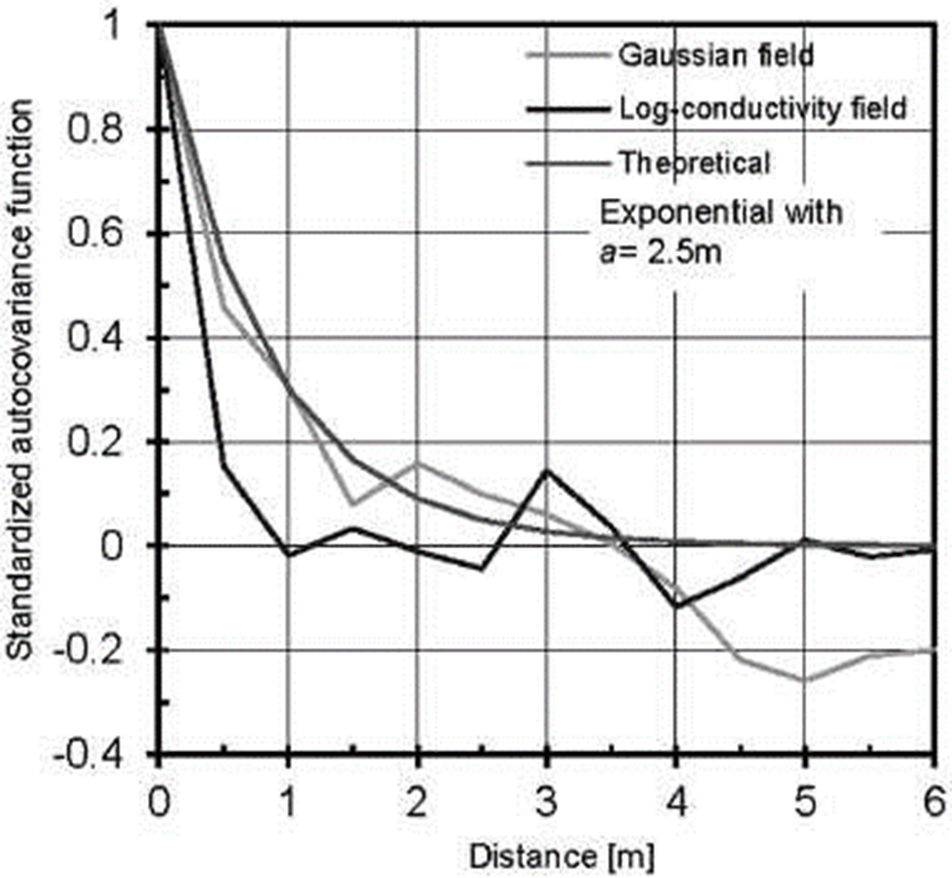
Figure 4. Standardized auto-covariance functions of the initial Gaussian field and reference log-conductivity field. An exponential function is also shown for comparison. 

In the present example, since y^ref (x) is normally distributed, k_s (x)=exp(y^ref (x)) is lognormally distributed with expected value m_Ks =0.315 m/day and variation coefficient CV_Ks = 1.31. Conductivity fields with lognormal univariate distributions and asymmetric spatial correlation are considered to be more representative of natural porous media (Gómez-Hernández and Wen, 1998; ^{Journel and Zhang, 2006}). Specific storage coefficient is assumed to be equal to 0.001m-1 throughout the porous medium.

Using the reference field of conductivities, groundwater head responses are generated by solving a transient flow condition with finite elements ^{(Smith and Griffiths, 2004)}. At t=0 days, the initial distribution of heads is hydrostatic. At t>0 days, hydraulic head decreases with time at a rate of 0.15 m/day during 150 days at the lower boundary. For the purpose of the present numerical example, the distribution of heads at t=90 days is assumed to be the initial condition (denoted as t=0 days in Figure 5 and henceforth). It is further assumed that groundwater head responses are available at times t=3, t=18 and t=60 days at the two locations indicated in Figure 5. Thus, two histories with three hydraulic head values are generated. These indirect, informative variables of the hydraulic conductivity of the reference field are considered available transient piezometric observations. At each one of these three times, the update step of the tEnKF scheme is performed.

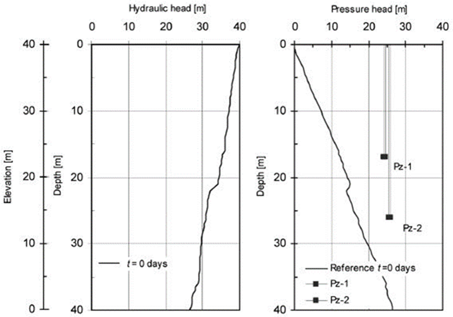
Figure 5. Profile of hydraulic heads in the reference field at t=0 days. The depths of the tips of two piezometers (Pz-1 and Pz-2) are indicated with filled squares. 

The reference field is sampled at four locations indicated in Figure 3c and the values are considered direct log-conductivity measurements. The mean and variance of the set of sampled values are reported in the same figure. Observe that these statistics overestimate the mean and variance of the reference field. Observe also in Figure 4 that an exponential auto-covariance function with correlation scale a=2.5m overestimates the correlation scale of the reference field as well. The sampled mean and variance, as well as the auto-covariance function mentioned above, are used to simulate two thousand unconditional multi-Gaussian log-conductivity realizations. Since the realizations are multi-Gaussian, they do not exhibit the asymmetric spatial correlation structure of the reference field ^{(Journel and Deutsch, 1993)}. This set of log-conductivity fields attempts to model a situation in which the mean value, variance and auto-correlation function of the reference field are only roughly estimated a priori and the asymmetry of this field is ignored. It represents, in fact, the prior uncertainty about spatial variability of the conductivity in the porous medium.

The chosen number of simulated realizations ensures the stability of the following two error measures, according to preliminary computations:

where n is the number of log-conductivities in the flow domain, y*(x i) is the estimated mean log-conductivity at location x _i , and y^ref (x _i ) is the reference log-conductivity also at location x _i .

The SPREAD is computed as:

where Sen2(xi) is the variance of the estimation of the log-conductivity at location x _i computed statistically over the ensemble of realizations.

It is worth mentioning that RMSE is a measure of the difference of the means of the estimated and reference fields and SPREAD is a measure of the dispersion of the estimated field around the reference field. Therefore, they can be viewed as measures of accuracy and precision of the estimations, respectively.

Results and discussion

Effect of the Gaussian transformation

Figure 6 illustrates the Gaussian transformation process of the hydraulic head at an arbitrarily selected node before the first update step. In general, the shape of the local distributions depends on the location of the node in the flow domain and on the boundary conditions of the problem at hand. In all cases, the local distribution functions can be transformed into Gaussian distributions by building local Gaussian anamorphosis functions numerically, as explained earlier. As can be seen in Figure 6(a), although the original values exhibit a skewed distribution, the transformed variable becomes symmetric around the mean showing the well-known bell-shape of the Gaussian anamorphosis (Figures 6b and 6c).

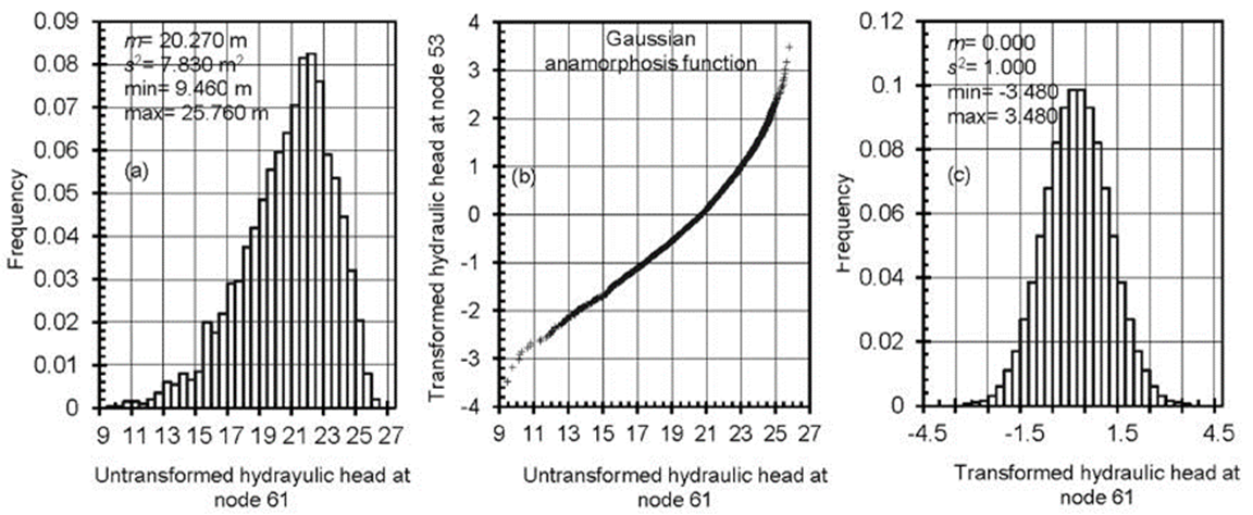
Figure 6. Gaussian transformation of hydraulic heads at node 61: a) Histogram of untransformed hydraulic heads, b) Gaussian anamorphosis function (with zero mean and unity variance), c) Histogram of hydraulic heads after the Gaussian anamorphosis. 

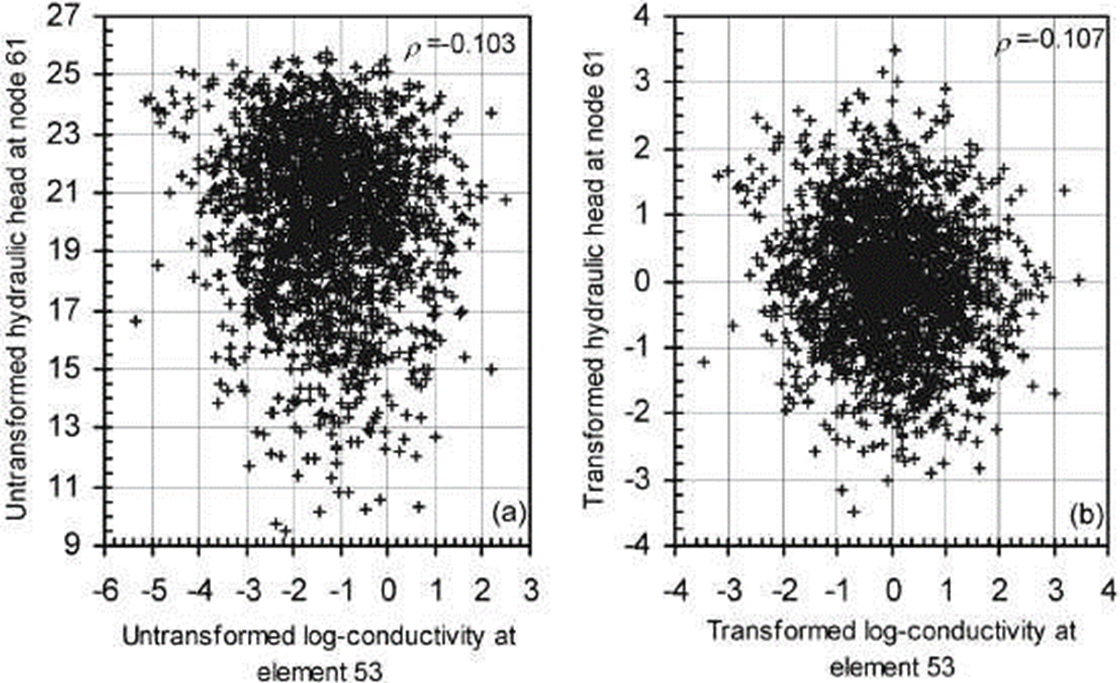
Figure 7 represents the relationship between log-conductivities and heads at arbitrarily selected locations, before (Figure 7a) and after (Figure 7 b) applying the respective Gaussian transformations. Given that the Gaussian transformation is monotonous, the bivariate characteristics of the dependence, such as the correlation structure at different percentiles, are not modified ^{(Deutsch and Journel, 1992}; ^{Chilès and Delfiner, 1999)}. However, the linear correlation coefficient, which depends on the kind of marginal distributions of the random variables, might be different before and after transformations. In the particular case of the variables at the locations indicated in Figure 7 (at the upper right corner of each figure), this coefficient presents nearly the same value before and after transformations. Therefore, the implicit pseudo-linearization effect associated to the Gaussian anamorphosis reported by ^{Shöniger et al. (2012)} should be considered application dependent.

Figure 7. Relationship between log-conductivity and hydraulic head at two arbitrary selected locations (r is the Pearson correlation coefficient): a) Before the Gaussian transformation of both variables, b) After the Gaussian transformation of both variables. 

Effects of conditioning on log-conductivities alone

The impact of conditioning realizations of log-conductivities to direct measurements only is analyzed. Figure 8 displays comparisons between the reference field of log-conductivities and the mean of the conditional realizations of log-conductivities. Contrasting both fields, it is observed that at the measurement locations the conditional value is the measured value.

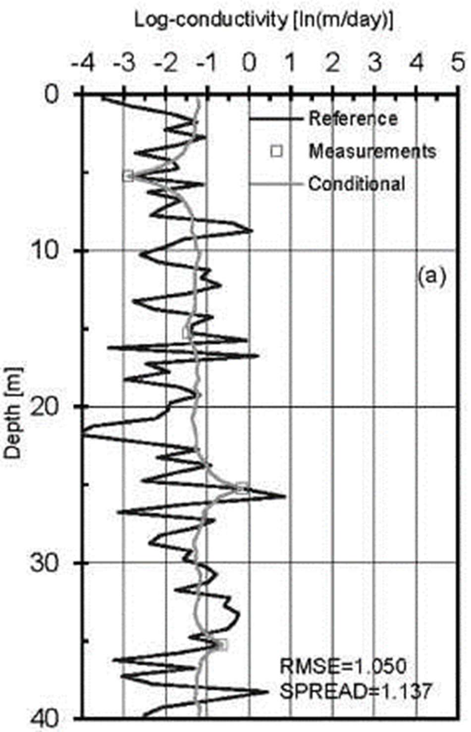
Figure 8. Log-conductivity fields conditional to log-conductivities alone. The reference field is also shown. 

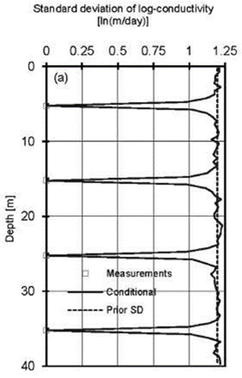
Figure 9 reproduces profiles of standard deviations (uncertainty) computed with the conditional realizations of log-conductivities. Observe that the effect of conditioning is to reduce, overall, the prior uncertainty and to collapse it to zero at the locations of the measurements.

Figure 9. Profiles of conditional standard deviations of log-conductivities with respect to depth (empty squares indicate the locations of known values). 

Effects of conditioning on log-conductivities and transient heads

In what follows, the additional impact of conditioning the realizations of log-conductivities to transient heads responses is examined. Comparisons of the reference field of log-conductivities with the mean of the conditional realizations of log-conductivities of the tEnKF at times t=3, t=18 and t=60 days are shown in Figures 10a, b and c, respectively.

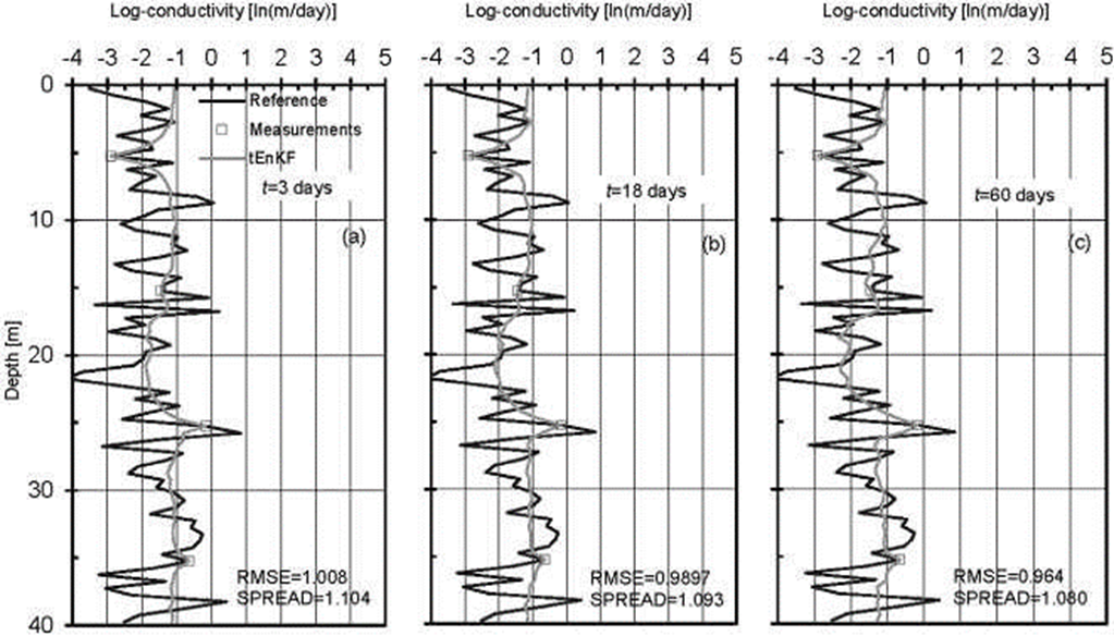
Figure 10. Log-conductivity fields conditional to histories of hydraulic heads with the tEnKF method. The reference field is also shown: a) At t=3 days, b) At t=18 days, c) At t=60 days. 

Contrasting the RMSE and SPREAD values shown at the bottom right corner of Figure 10a with the same two error measures shown in Figure 8, it can be observed that the estimation of the hydraulic head field becomes more accurate and precise after assimilating the first pair of measured hydraulic heads with the tEnKF. Further improvements in the estimation of the reference field are observed as more measured hydraulic head data are assimilated. For instance, the RMSE and SPREAD values for the conditional mean log-conductivity field of the tEnKF at time t=60 days are 0.964 and 1.080, whereas before the filtering process they were equal to 1.050 and 1.137, respectively. The accuracy of the estimation with the tEnKF can be attributed to the fluctuations that occur between measurements which follow the variability of the reference medium more closely. However, it should be recalled that the RMSE and SPREAD values measure the quality of the local estimation only, i.e. they do not indicate anything about the quality of the multivariate estimation. Bivariate empirical copulas can be used to perform this evaluation ^{(Bárdossy and Li, 2008)}.

The standard deviation profiles calculated with the realizations of log-conductivities of the tEnKF are reported in Figure 11. The overall uncertainty decreases as longer groundwater head records are incorporated into the update step, except at the locations of direct measurements where uncertainty is zero at all times. The Figure shows that uncertainty is smaller around depths of 17 m and 26 m (where the tips of the two piezometers are located) than at other depths.

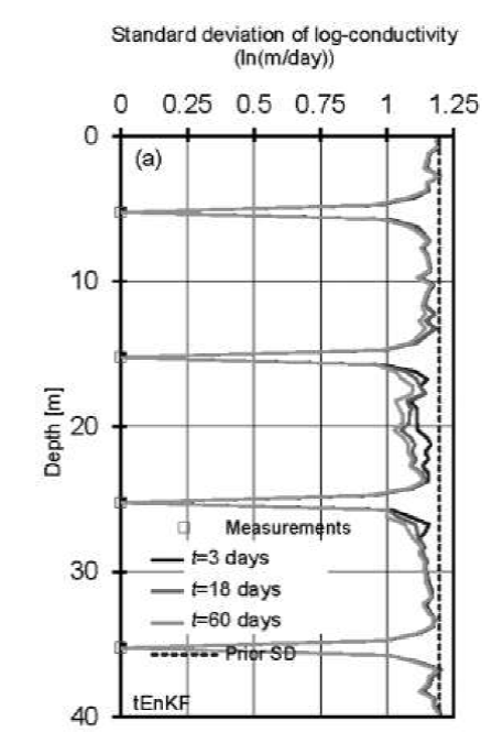
Figure 11. Profiles of conditional standard deviation of log-conductivities with respect to depth at different times (empty squares indicate the locations of known values). 

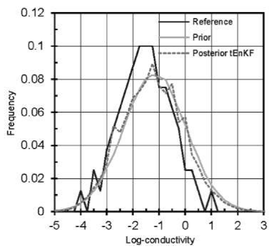
Figure 12 displays the frequency distributions of log-conductivities of the reference field and of the prior and posterior ensembles at the end of the conditioning process. Recall that the mean value of the conductivity of the reference field was overestimated by the prior random field; hence, the distribution function of this field is located to the right of the field’s frequency function. Looking at the distributions of the posterior fields, it is observed that they exhibit some features of the reference frequencies (like some of the “peaks” of both branches) and that they are slightly displaced toward the left of the frequencies of the prior random field. This result illustrates the attempt of the filter to lead the prior frequencies toward the reference frequencies when a small number of instruments and short records of measured hydraulic head responses (t=3, t=18 and t=60 days) are used in the conditioning process and when the initial representation of the asymmetric correlation structure of the true field is ignored by the prior random field model. Although there is a benefit, the degree of improvement of the initial approximation should be further investigated because the depth and distance between instruments, as well as the times at which observations are available, and the length of the histories of hydraulic head responses may also have an effect on the results.

Figure 12. Frequency distributions of logconductivities of the reference field, set of prior realizations and sets of posterior realizations at t=60 days. 

Conclusions

This paper proposed that in order to evaluate the performance of tEnKFs in synthetically generated fields of the hydraulic conductivity, it is necessary to take into account the risk of introducing a systematic bias in the spatiotemporal evolution of the hydraulic head field by incorporating prior knowledge with a multi-Gaussian conductivity correlation structure, and by adopting a reference field with asymmetric correlation structure. This setting aims to offer a truer representation of common situations in practice in which the first two moments and the auto-covariance function of the real field are roughly known, but the asymmetry of the spatial correlation structure of that field is unknown.

As an example of the proposed approach, hydraulic conductivities were identified using the tEnKF by solving a one-dimensional, single phase flow problem in a continuous random porous medium. Three effects on the reproduction of the reference field were evaluated: the effect of the Gaussian transformation process, the effect of incorporating only measured hydraulic conductivities and the effect of incorporating measured hydraulic conductivities and hydraulic heads data. The results of this example indicate that when the asymmetry of the spatial correlation structure of the reference field was unknown a priori, the tEnKF was still capable of improving the initial approximation. However, no definitive conclusions can be drawn from this study in terms of the performance of tEnKF under this constraint since the degree of improvement of the initial approximation may further depend on the configuration of the array of instruments, the times at which observations are available and the length of time series of hydraulic heads.

Further research is needed to fully assess the performance of the EnKF with transformed data. For example, its effect on the reproduction of the multivariate spatial dependence of a non multi-Gaussian reference field using a multi-Gaussian random field model of conductivities in the prior approximation should be explored