Introduction

Analysis of seismic data from an array of sensors has been very useful to study wave propagation, particularly, to discriminate between natural earthquakes and underground nuclear explosions. With this purpose, in the 1960s and 1970s, the use of large aperture seismic arrays, generally designed for optimal detection of regional and teleseismic events, was widely spread. An example was, the LASA (Large Aperture Seismic Array) located in Montana (USA), an array of 525 shortperiod seismometers covering a radius of 100 km by groups of 25 sensors concentrically arranged. In each group, the sensors were equally distributed in an area of 3.5 km radius (^{Green et al., 1965}). Another large aperture arrangement was NORSAR, located north of Norway. With a similar configuration, NORSAR consisted of 132 short-period seismometers and covered a radius of 50 km. The sensors of these two arrangements recorded only the vertical component of the movement. Over the years, the use of arrays of seismic sensors of a single component has been very helpful in the first arrival detection and in the identification of apparent velocities and directions of the fields of incident waves. ^{Ringdal and Husebye (1982)} made a detailed review of these experiences. Since the first experiences, diverse theories have been proposed aimed to characterize the motion in terms of power density estimators in the ƒ - k domain.

In general, it has been assumed that the motion, recorded by an array, is a stationary random process with zero mean and standard deviation σ. When the motion is coherent, the variance of the process is a good approximation estimator of the power spectral density (^{Yaglom, 1962}). However, the resolution of this conventional approximation estimator is rapidly lost when the coherence of records decreases. As a result, high resolution approximations estimators have received more attention. One of them is the maximum likelihood filter (^{Capon et al., 1967}; ^{Capon, 1969}; ^{Kværna and Doornbos, 1986}), especially recommended for irregularly distributed arrays.

In the analysis of tele seismic data, it is common to classify the wave field’s components in terms of their apparent velocities (^{Aki and Richards, 1980}). In many cases, the particle motion analysis, as the one proposed by ^{Jurkevics (1988)}, can be used as a complement in the recognition of wave’s type. ^{Mykkeltveit et al. (1983)} note that this procedure allows to distinguish prominent phases in seismograms. The ƒ - k analysis applied to seismic data is also known as Multichannel Analysis of Surface Waves method (MASW; see ^{Park et al., 2007}).

The accelerograms of the Michoacán Earthquake of September 19, 1985 (Ms 8.1) recorded by some stations within the Mexico City Valley showed, among many other aspects, the coherence between records (^{Campillo et al. 1989}) and allowed to identify the presence of conspicuous waves of long and short period. This fact served to calibrate a regional crustal model. After this earthquake, the MCAN was deployed. The ensuing strong-motion recorded in Mexico City, clearly show large amplifications beyond the level predicted using simple onedimensional (1D) shear models (^{Sánchez Sesma et al., 1988}; ^{Kawase and Aki, 1989}). This strongly suggests significant lateral effects of three-dimensional (3D) nature. The spatial variability and polarization of observed ground motion have been interpreted as 3D effects (^{Pérez-Rocha et al. 1991}; ^{Sánchez-Sesma et al., 1993}).

Currently, the MCAN has over 70 three-axial surface accelerometers irregularly distributed in the city; the area covered is of approximately 600 km². More than 170 intense and moderate events, mainly from the coast, have been recorded by this network.

In this work, seismic records of motion caused by a well recorded earthquake in Mexico City Valley (March 20, 2012), were analysed. The results reveal the propagation of wave components across the Valley in both longitudinal and transversal motions. The characteristics of these components allow identifying the interaction of incoming waves with the geological structure of the Mexico City Valley.

In order to estimate the power spectra of the kinematic wave components in the ƒ - k domain, a wave decomposition was performed, implementing a maximum likelihood filter, based on the Helmholtz theorem and the ^{Capon method (1969)}. A spectral representation that displays amplitudes, directions and propagation velocities of waves with longitudinal and transversal polarization allows interpreting the behaviour of waves trapped in a sedimentary environment.

Power spectral density of the kinematic components of a wavefield

Fourier analysis in time domain is an usual tool in seismology and it is the keystone of many developments in mathematical-physics. Its extension to space-time configurations in which one or various coordinates are dealt with analytically, shows the great resolving power of Fourier analysis. This is the case when it is used in regular arrays. In many instances it comes out that arrays in which data is avilable, are not regular and even an approximate description is desirable.

An analysis of the kinematic components of a vector wavefield is presented, starting from the continuous description of a vector field in the space-time frame and using the results within the frame of approximate spectral estimation based on the maximum likelihood theory of ^{Capon (1969)}.

Power spectral density

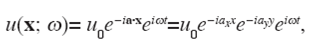
The displacement field u (x; ω) due to the propagation of a harmonic plane wave is given by:

1

where u₀=u₀ ( ω ) is the spectrum of the signal with information of its waveform. Here a = (a_x, a_y)^T = ( ω / c) n is the wavenumber vector with components, a_x = ωn_x / c and a_y = ωn_y / c; ω is the angular frequency, and c the wave propagation velocity. The wave direction is given by the vector n = (n_x, n_y)^T. Finally, x = (x, y)^T is the position vector.

After the spatial Fourier transform, the field in wavenumber domain is:

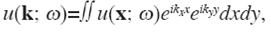2

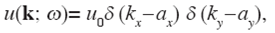3

where δ (⋅) is the Dirac’s Delta function:

4

Therefore, the spectrum in the wavenumber domain given by eq. (2) is theoretically zero for the coordinates indicated by the vector k = (k_x, k_y)^T that differs from a = (a_x, a_y)^T. This represents a prominent peak in the spectrum and leads to determine the direction and velocity of propagation of a plane wave.

The velocity c and the azimuthal direction of propagation θ are obtained with the following equations:

5

6

It is clear that the azimuth is measured with respect to North-South (NS) direction. ^{Capon (1969)} designed a high resolution filter to estimate the ƒ- k power spectral density |u(k; ω )|² when the field is only known in M sensors distributed in the x-y space. This estimation allows the undistorted passage of any monochromatic plane wave that propagates with wavenumber vector a:

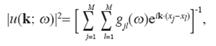7

where g_jl (ω) is the jl element of the matrix G=F⁻¹ and F is the spectral correlation matrix; each element jl of F is given by f_jl( ω )=u_j (x; ω ) u_l*(x; ω ) (here * denotes complex conjugate).

Kinematic decomposition

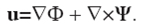
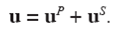
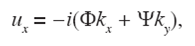
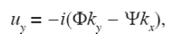
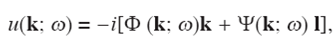
Assume that P waves (with longitudinal polarization of particle motion) and S waves (with transversal polarization of particle motion) propagate in a medium. According to the kinematic decomposition of Helmholtz, if θ and Ψ are the displacement potentials for P and S waves, respectively, with ∇⋅Ψ = 0, then the total displacements field is written as:

8

By definition u ^P=∇Φ and u ^S=∇×Ψ. Then, it can be written

9

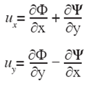
The total horizontal displacements in the plane x − y, admit the next representation:

10

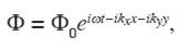
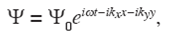
since Ψ= (0, 0, Y). If the potentials Φ and Ψ are harmonic and represented by:

11

12

Then, the components of the displacements field in the x and y directions acquire the forms:

13

14

If l=(k_y, − k_x)^T , the total field u(k; ω ) can be written as:

15

where k ⋅ l = 0.

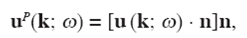
In this result, the propagation vectors associated with P and S waves are recognized parallel and perpendicular to the vector k, respectively. Moreover, the displacement field produced by P waves is the component of the total field in the direction of the vector k, whereas the field produced by S waves is the component of the total field in the direction of the vector l:

16

17

The unit vectors n and m indicate the directions of propagation of the wavenumbers k and l, respectively, and are given by,

18

19

where This kinematic decomposition is developed for the plane x - y, therefore the longitudinal component of Rayleigh waves is analogous to P waves in the above development. In the same way, the transversal component of Love waves is regarded as S waves.

Numerical example on a 2D space

The kinematic decomposition is validated in a 2D setting by simulating the propagation of two plane waves. Thus, two plane P and SV waves are considered with propagation velocities of 2.6 and 1.5 km/s, respectively. The respective azimuths are 60 and -20 degrees. Both waveforms are Ricker wavelets with characteristic frequency of 1 Hz.

The array used in this example is shown in Figure 1. It is composed by a random distribution of 30 stations in a square of 4 km x 4 km. The purpose of applying the ƒ- k spectral analysis in a random array with few stations is to check the strength of the kinematic decomposition formulation to describe the total field in longitudinal and transversal components.

Figure 2 displays the k_x - k_y diagrams of the longitudinal and transversal displacements, associated with the frequency of 1 Hz. The component distinctions emerge from the application of the separation vector described in eqs. (16) and (17).

Figure 1 Spatial array of 30 stations randomly distributed in a square of 4 km x 4 km. 

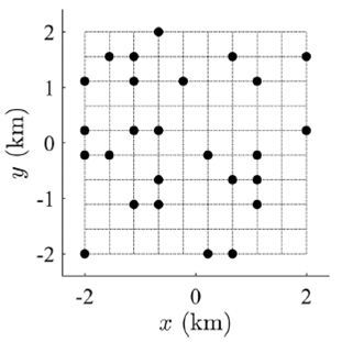
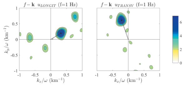
Figure 2 k_x − k_y diagrams of components longitudinal (u_LONGIT) and transversal (u_TRANSV) components, at left and right, respectively, associated to the frequency of 1 Hz for two P and SV plane waves propagating in a 2D space and crossing the array depicted in Figure 1. The black doted lines indicate the vector of the principal peak for each diagram. 

In each diagram, energy concentrations can be observed, associated with the incidence or emission of coherent waves observed in a large number of station arrays detected by this analysis. Using the wavenumbers (k_x, k_y) in which each peak is located, the wave propagation speed c, and direction, θ, can be determined by applying eqs. (5) and (6). The direction corresponds to the azimuth, which is measured from NS direction or in this particular case from axis. Therefore, k_x = (c/ ω ) sin θ and k_y = (c/ ω ) cos θ

Figure 2 clearly depicts a longitudinal wave located in k_x / ω = 0.32 km^-1 and k_y / ω = 0.2 km^-1, which represent a wave traveling with c = 2.63 km/s and θ = 58 degrees. A transversal wave is also observed in k_x / ω = -0.22 km^-1 and k_y / ω = 0.62 km^-1, which corresponds to a wave with c = 1.53 km/s and θ = -19 degrees. The description of these two waves from ƒ- k analysis exactly matches the initial parameters of the incident waves.

Numerical example on a 3D alluvial valley

In order to calibrate this kinematic decomposition, the surface field of an elastic 3D alluvial valley on an elastic half-space under the incidence of plane waves (P, SV, SH and Rayleigh) is separated in terms of longitudinal and transversal spectral motion. The reference results were computed with IBEM for the model presented by ^{Sánchez-Sesma and Luzón (1995)} for the scattering and diffraction of elastic waves by soft elastic inclusion models of alluvial deposits in an elastic half-space.

This is a closed irregular croissant-type alluvial valley (V) over a half-space (HS), depicted in Figure 3. The valley is 0.25 km depth, and is 2 km of longitude in its longest side. The free surface of both the valley and the half-space are assumed flat. The shear wave speeds are β_V = 1 km/s and β_HS = 2 km/s; the Poisson ratios are u_V = 0.35, u_HS = 0.25, and the mass densities satisfy p_V = 0.8 p_HS. A quality factor of 100 was assumed for both P and S waves inside the valley. The half-space has no internal attenuation.

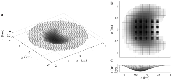
Figure 3 Synthetic model of a croissant-type alluvial valley. (a) Depict the 3D topography of the interface; (b) croissant plan view, where the location of the array is indicated with black dots, which is composed of a distribution of 20x20 equally spaced stations, and (c) valley’s lateral view. 

The array has 20 x 20 stations equally spaced (Δx = 0.0526 km) within a square. It is located inside the croissant valley on free surface as depicted in Figure 3 (b). Note that the right side of the array cross the valley’s edge. The side’s length of this square array is L = 1 km.

Both dimensional parameters: L in the studied direction, and Δx, control the confidence limits of the wavenumbers in the ƒ- k analysis. In an arbitrary array, the minimum wavenumber that should be analysed is: k_min = Δk/2π = 1/L, and the maximum wavenumber, or Nyquist (Nq) wavenumber, that should be studied is k_max = k_Nq/2π = 1/2 Δx. In this particular case, these two dimensional parameters are: k_min = 1 cycles/km, and k_max = 9.5 cycles/km.

We consider the incidence of a SV wave with θ = -10 degrees, and a Rayleigh wave with θ= 90 degrees, both of them with propagation velocity of 0.5 km/s. For the incoming waves Ricker wavelets with characteristic period equal to 0.33 Hz, was assumed. Synthetic seismograms are depicted in Figure 4.

The ƒ- k analysis in four time windows of 10 s with an overlap of 2 s: 0 - 10 s, 8 - 18 s, 16 - 26 s, and 24 - 34 s (see Figure 4) was applied, in order to follow waves both incident or emitted by the edges of the valley, and identify their type, velocities and directions of propagation.

The windows’ length depends on the desired level of detail in the analysis. Generally, the records’ total duration can be used, but waves with large amplitudes overwhelm coherent waves with low amplitudes in the coda and thus prevent their detection. The window’s resolution depends on the signal frequency, the likely apparent velocity and the array’s spatial dimension. It is recommended that the time window contains at least three wavelengths to allow that the propagating waveform is contained in the selected window, so that their spectrum amplitude and phase are well retrieved.

For each time window we construct kinematic spectra of the amplitudes, velocities and directions of propagation for the longitudinal, transversal and vertical displacements of the wave field. These spectra are constructed from the wavenumbers (k_x, k_y) of the peaks detected in the k_x - k_y diagrams for each frequency using eqs. (5) and (6) to compute c and θ, respectively.

The vertical component is used jointly with the longitudinal one to corroborate the possible presence of Rayleigh waves. The propagation velocities and directions of these waves must be equal in both the longitudinal and vertical components, and in the amplitudes, vertical component must be slightly larger, at least for a prevailing fundamental mode.

At the kinematic spectra for the time window 0 - 10 s depicted in Figure 5 (a), using both the longitudinal and vertical components, a prominent Rayleigh wave i can be seen s observed, with frequency between 0.3 and 0.4 Hz, c = 0.4 km/s approximately and θ = 90 degrees. From the transversal component, a S wave of f = 0.35 Hz, c = 0.5 km/s and θ = -20 degrees can be seen. In the same time span, another S wave with ƒ = 0.3 Hz, c = 0.5 km/s and θ = 135 degrees, almost opposite to the previous one, can also be seen .

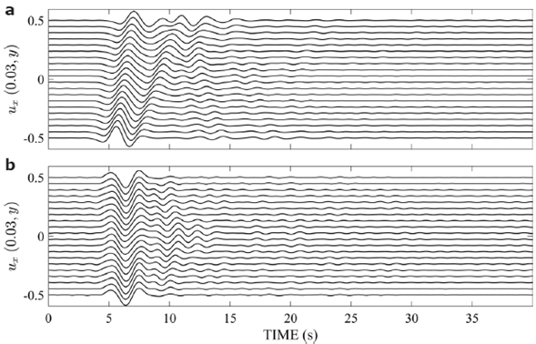
Figure 4 Displacements at stations located at x = 0.03 km of the synthetic model shown in Figure 3 subjected to the incidence of two plane waves: (a) a SV with θ = -10 degrees, and (b) a Rayleigh wave with θ = 90 degrees. 

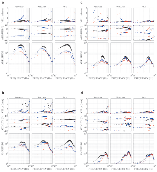
Figure 5 Kinematic spectra of longitudinal (u_LONGIT), transversal (u_TRANSV), and vertical (u_VE) displacements of the 3D synthetic model depicted in Figure 3, corresponding to the time windows (a) 0 - 10 s, (b) 8 - 18 s, (c) 16 - 26 s, and (d) 24 - 34 s. The propagations velocities are at the top, the azimuths are at the middle and the amplitudes are at the bottom. The markers’ types indicate the relevance of the peaks detected in the k_x − k_y diagrams; thus, higher amplitudes are indicated with black circles, followed by blue triangles and then by red squares. The markers’ sizes depend on the amplitude of each frequency normalized with respect to the maximum amplitude for all frequencies. 

Figure 5 (b) correspond to time window between 8 and 18 s. It reveals a principal S wave ƒ = 0.35 Hz, c = 0.4 km/s, and θ = -10 degrees. No prominent waves in the longitudinal component can be seen in this time window.

The results depicted in Figure 5 (c) and (d) correspond to time windows 16 - 26 s and 24 - 34 s, respectively, and reveal very interesting patterns of interference of the refracted waves inside the basin and, in some cases, significant emission of waves is observed.

From Figure 5 (c), that covers time window 16 - 26 s, we can see the propagation of initial waves with θ = 0.5 Hz in the three components. In the longitudinal component it travels with c = 0.3 km/s, and θ = 45 degrees. In the transversal component, it revels three S waves with c = 0.3 km/s, in a range of directions of approximately 5, 65 and 130 degrees.

From Figure 5 (d), corresponding to time window 24 - 34 s, we can see in the longitudinal component: the propagation of a wave with a range of frequencies between 0.7 and 0.77 Hz, with c = 0.3 km/s, and q = -145 degrees, i.e., it is traveling backward. With the same frequencies and velocity but with smaller amplitudes there are two waves propagating with q = 17 and 57 degrees, almost opposite to the first one.

There is also a wave with ƒ = 0.4 Hz, with c = 0.35 km/s, and q = 40 degrees. In the transversal component, the propagation of three waves is spotted for an interval of frequencies between 0.7 and 0.77 Hz, with velocities in the interval of 0.27 and 0.32 km/s, and directions of -30, 11 and 125 degrees. Moreover, one can infer the propagation of a transversal cylindrical wave with ƒ = 0.5 Hz, velocity around 0.3 km/s, coming from N135E, i.e., traveling backward.

We attribute the changes in the propagation directions and the presence of several peaks in the power spectra as an evidence of the scattering and diffraction of the incident wave field by the basin’s edge.

Figure 6 shows the k_x - k_y diagrams associated to only one frequency for each of the four time windows analyzed. The various panels presented give support to the kinematic spectra depicted in Figure 5.

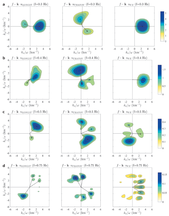
Figure 6 Diagrams in the k_x − k_y space for the four studied time windows (a-d). Each one is associated to the spectra shown in Figure 3. The diagrams correspond to a single frequency. For each case, the window limits and the associated frequency are: (a) 0 - 10 s for ƒ = 0.35 Hz, (b) 8 - 18 s for ƒ = 0.35 Hz, (c) 16 - 26 s for ƒ = 0.5 Hz and (d) 24 - 34 s for ƒ = 0.75 Hz. In each row, longitudinal (u_LONGIT), transversal (u_TRANSV) and vertical (u_VE) displacement amplitudes are at the left, center, and right, respectively. The black doted lines indicate the vector of the principal peaks for each diagram. 

Analysis of seismic data recorded by MCAN

The important site effects that occur at Mexico City subsoil due to earthquakes, especially the long duration and the increased amplitudes on seismograms recorded in free surface inside de City, lead to the search of ways to improve the understanding on the mechanisms that control these phenomena.

In this study, we apply a time-space spectral analysis to obtain in the ƒ- k domain, spectral power densities of the strong ground motion recorded by the MCAN. This method will allow us to figure out the behaviour of the incident and emitted wave fields within the Valley.

Figure 7 shows the distribution of the MCAN as well as the Geotechnical Zonation location. Two parameters control the confidence limits of the wavenumbers in the ƒ- k analysis. They are: the array length in the studied direction, L = 30 km for both sides, and the average separation between stations, Δx = 3.33 km which comes from the maximum instrument density located in the central area of the network. Therefore, taking into account these two values, the minimum wavenumber that should be analysed is k_min = Δk/2π = 0.033 cycles/km, and he maximum wavenumber, or Nyquist (Nq) wavenumber, that should be studied is k_max = 0.15 cycles/km.

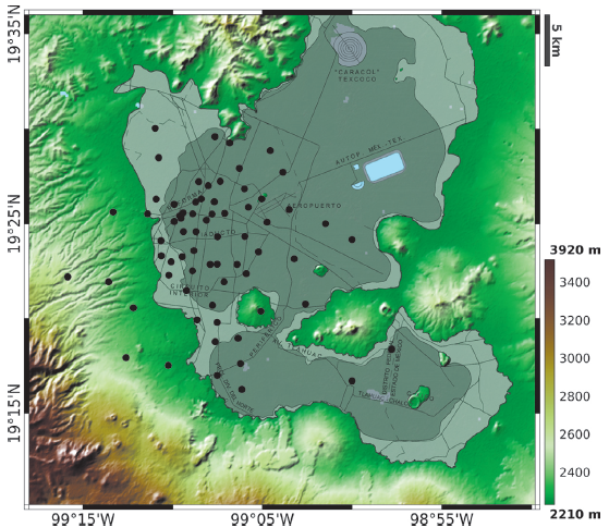
Figure 7 Elevation map of Mexico City Valley and Geotechnical Zonation. The black line inside the basin delineates the edges of the lacustrine deposits. Within these edges the Lake Zone is shaded in solid dark grey, and the Transition Zone is represented by solid light grey. Outside these edges, the Hill Zone begins in green (above 2,300 m.a.s.l.). The black dots indicate the locations of Mexico City Accelerometric Network (MCAN). 

Previous studies (^{Campillo et al., 1989}, and ^{Sánchez-Sesma et al., 1993}) identified, in the vertical component of the displacements recorded inside Mexico City Valley, crustal surface waves coming from the Mexican subduction zone. ^{Campillo et al. (1989)} identified two prominent surface waves with characteristic periods of 0.1 Hz and 0.33 Hz in the records produced by the September 19, 1985, Michoacán earthquake (Mw 8.1) and proposed a cortical model that allowed them to postulate that the long-period waveform of 0.1 Hz corresponds to the fundamental mode of Rayleigh surface wave, and is preceded by a short-period waveform of 0.33 Hz which is associated with the propagation of higher modes of Lg surface waves. Sanchez-Sesma et al. (1993) detected also these two particular waves in the MCAN’s records of the April 25, 1989, earthquake (Mw 6.9) by applying the ƒ- k analysis.

In this study, a more recent event (with characteristics similar to the ones mentioned above) was selected to be analysed, i.e., large magnitude with its epicenter in the Mexican subduction zone, and with important site effects when arriving to Mexico City Valley. The event is the March 20, 2012, earthquake (Mw 7.4) recorded at 60 MCAN stations.

The displacements in six MCAN arbitrary sites due to this event after the double integration of the accelerograms, appear in Figure 8. In the vertical displacement of the set of records, it is also possible to observe two conspicuous incidences: Rayleigh (ƒ = 0.1 Hz) and Lg (ƒ = 0.33 Hz) surface waves between 80 and 130 s.

A successive ƒ- k analysis of time windows can determine the wave field behaviour of the records at late times, which are very likely the result of multi-pathing inside the Valley, i.e., the product of waves interaction with the edges of the basin. This interpretation should be subjected to closer scrutiny considering more realistic cortical models and the correlation with surficial geological structures.

In this sense, the displacement spectral densities and the kinematic decomposition in longitudinal and transversal components, for four time windows: (a) 80 - 130 s, (b) 120 - 170 s, (c) 160 - 210 s, and (d) 200 - 250 s were estimated. The last three time windows correspond to the early coda of the earthquakes.

Figure 9 displays the kinematic velocity spectra, direction of propagation and Fourier amplitudes for the four time windows in the frequency band between 0.06 and 0.6 Hz. These spectra were constructed with the three maximum peaks of the diagrams for each frequency. This representation allows identifying the spectral characteristics of the k_x - k_y wave field components.

Figure 9 (a) shows three representative peaks in all components at frequencies equal to 0.11, 0.15 and 0.33 Hz. The first peak with relevant amplitudes can be observed in an interval of frequencies between 0.1 and 0.13 Hz which propagates in direction around -10.3 degrees, with velocity equal to 2.9 km/s. This peak appears in the longitudinal and vertical direction, which strongly suggests that it is the fundamental mode of Rayleigh waves. Another representative peak occurs at 0.33 Hz in the transversal component, which propagates at -13 degrees with a velocity of 3.6 km/s. We associate this wave with Lg surface waves. The direction of propagation of these two waves is very close to the epicentral direction N10W. This fact suggests that they are incident waves coming from the source. The inferred type of wave and velocities matches with the ones identified by ^{Campillo et al. (1989)}. The speed and direction of propagation of these two wave episodes are directly seen on seismograms. Therefore, we consider it as a validation of the method that can track waves crossing the Valley and are not clearly detected on seismograms. Another identified waves episode in the transversal component corresponds to the ƒ = 0.15 Hz, with c = 2.8 km/s, and θ = -18 degrees.

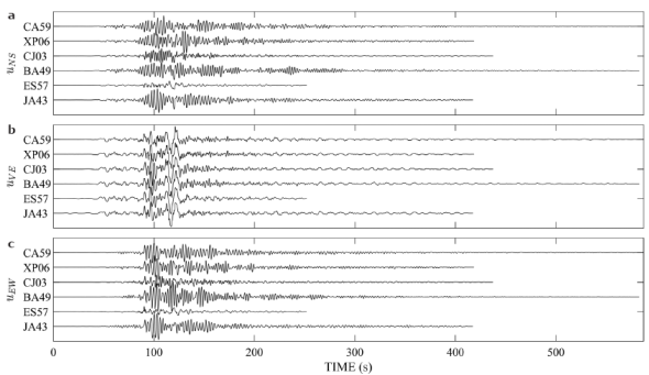
Figure 8 Displacements of the March 20, 2012, earthquake after the double integration of the accelerograms observed in six MCAN arbitrary stations. (a) North-South component (u_NS), (b) Vertical component (u_VE), and (c) East-West component (u_EW). The stations’ names are indicated on the left of each trace. The u_VE traces are scaled by a factor of 5. 

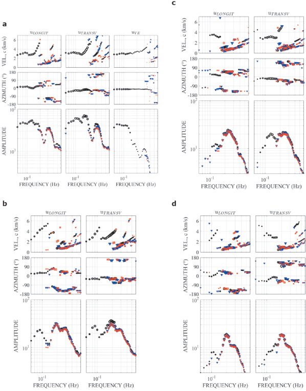
Figure 9 Kinematic spectra of longitudinal (u_LONGIT), transversal (u_TRANSV), and vertical (u_VE) displacements observed in the March 20, 2012, earthquake (see Figure 8), corresponding to the time windows (a) 80 - 130 s, (b) 120 - 170 s, (c) 160 - 210 s, and (d) 200 - 250 s. Because of the low amplitudes of the vertical components, the only one depicted is in case (a). The propagations velocities are at the top, the azimuths are at the middle and the amplitudes are at the bottom. The markers’ types indicate the relevance of the peaks detected in the k_x − k_y diagrams; thus, higher amplitudes are indicated with black circles, followed by blue triangles and then by red squares. The markers’ sizes depend on the amplitude of each frequency normalized with respect to the maximum amplitude for all frequencies. 

Figure 9 (b), (c) and (d) which correspond to the early coda of the seismograms show the kinematic spectra of the longitudinal, transversal, and vertical components. It can be seen, in the interval of frequencies between 0.2 to 0.5 Hz, comparable amplitudes in the three kinematic components with significant changes in directions and velocities of propagation. As in the synthetic model case of a croissant-type alluvial valley, we attribute this behavior of the wave field to an evidence of the diffraction of the incident field due to its interaction with the edges of the basin, and in this real case, also to the multipath that waves take from the epicenter to the Mexico Valley. Moreover, for these frequencies our results suggest that the field is composed by surface waves higher modes, Rg and Lg, in agreement with ^{Campillo et al. (1989)}.

The phase velocities obtained from the analysis of the MCAN data, in the range of frequencies between 0.1 to 0.5 Hz are consistent with those obtained from the dispersion curves of the accepted theoretical crustal models for central Mexico (see ^{Gaite et al. 2012}). A discontinuity in the experimental results about ƒ = 0.2 Hz, both in phase velocities and propagation directions, suggests a possible conversion of surface wave to higher Rg and Lg modes, probably generated on the south edge of the Transmexican Volcanic Belt. Apparently, the cortical paths from this geological structure towards the Valley of Mexico, is very efficient for the propagation of these mode shapes. This follows from the conspicuous amplitudes of the power spectrum of these forms of propagation and could be related with the regional amplification identified by ^{Ordaz and Singh (1992)}.

The resolution of the power density estimators decreases rapidly for frequencies larger than about 0.5 Hz. This is a consequence of the decrease of the signal-to-noise ratio mainly because the minimum distance between MCAN sensors is around 3 km and wavelengths are less than 6 km, because waves propagate typically with horizontal velocities less than 3 km/s.

Conclusions

The importance of estimating the ƒ- k power spectral densities within the analysis of wave propagation from data of an array of sensors has been discussed. Higher resolution filters based on ^{Capon’s (1969)} maximum likelihood estimators, were applied. We have also proposed a kinematic decomposition of the wave field in longitudinal and transversal components, which permits to observe the directions, velocities, and polarizations of the surface displacement field.

For validation, the kinematical decomposition was implemented for two synthetic models, in 2D and 3D configurations, respectively. The results were successful because the parameters of the incident wave field like wave type, velocity and direction of propagation were well identified. The 3D model was a croissant-type alluvial valley, in which the influence of basin geometry was identified in surface motion.

For the March 20, 2012, earthquake recorded by the MCAN, the analysis and the kinematic decomposition in longitudinal and transversal components permitted to detect the propagation of waves in different time windows. In early times of seismograms, the incident wave field is recognized, while for late times, the analysis made possible to follow the variety of waves with frequencies between 0.2 and 0.5 Hz that are propagating across the Valley. They may be the result of the interactions of the incident wave field with the edges of the basin. The analysis of early times also reveals locally generated surface waves. They are somehow shadowed by incident waves, but their distinct azimuths may allow their detection. These facts may clarify the retrieved surface waves from correlations of strong ground motion for pairs of observers inside the Valley.