


 nueva página del texto (beta)
 Inglés (pdf)
 Artículo en XML
 Referencias del artículo
 Enviar artículo por email
 Citado por SciELO
  Similares en
SciELO
Similares en
SciELO 
 Permalink
Introduction
The Santos Basin is located in the southeastern region of the Brazilian continental margin, between 23o00'S e 28o00'S, and extends up to the bathymetric depth of 3.000 m (Figure 1). It has about 350.000 km2, covering the coastal states of Rio de Janeiro, São Paulo, Paraná and Santa Catarina (Moreira et al., 2007). The basin is bounded to the north by the Cabo Frio High and to the south by the Florianópolis lineament.
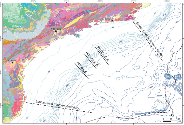
Figure 1 Location of Santos Basin. The continent-ocean boundary, according to Cainelli and Moriak (1999) is represented by the dashed line and bathymetric isolines are represented by blue the blue lines. The studied profiles A,B and C are also shown.
The formation of this basin is related to the opening of Supercontinent Gondwana, from the Lower Cretaceous (± 135 Ma), which resulted in the separation of South American and African continents. During the Neoaptian, the deposition of thick evaporite packages, generally composed of halite and anhydrite. This evaporite sequence was deposited due to the high rate of thermal subsidence in the Santos Basin, coupled with a gradual water intake isolated sea by proto-Gulf South (Gamboa et al., 2008).
In the Upper Cretaceous (Santonian-Campanian), due to reactivation of old faults of the basement, there was an uplift in the continental area, causing a remarkable siliciclastic erosion and progradation of clastic wedges into the basin, that was in subsidence process in the same period (Macedo, 1987 and 1989; Almeida and Carneiro, 1998). This siliciclastic progradation during this period, was responsible for the deformation of the evaporite packages and for moving these packages into the depocenter of the basin, providing a thick layer in the region known as Plateau of São Paulo, where the seismic investigations show remarkable presence of halokinetic structures, such as diapirs and salt walls.
The evaporite packages in the Santos Basin show interleaves with halite domain and a few layers of anhydrite. Both have constant seismic velocity with burial and thus, the seismic amplitude contrast between layers of these salts and adjacent sediments depends only on their the acoustic properties. On the other hand, the density contrast of sediments may vary with depth (Jackson & Talbot, 1986). The halite has a high seismic speed but a low density, around 2.17 g / cm3. The anhydrite has a high speed and a high density value, of approximately 2.98 g / cm3 (Bassiouni, 1994). Due to these differences of density, interpreting seismic data set using the gravity anomaly data can be a good solution to identify these different types of salt, modelling more precisely the evaporite packages and the adjacent sedimentary packages.
Previous studies as Mio (2005) and Lima & Mohriak (2013), show modelled crustal structures in the region of the Santos Basin from seismic data and gravity data, originating geological models for the studied regions. These works focuses primarily on modelling the seismic data and subsequently obtaining the adjustment together with the gravity data. In 2D seismic data, the top basement surface, due to the low resolution of the data at depth, is performed with less precision than shallower and more defined surfaces, such as the top and the base of the salt. In the case of the Moho, most of the time the horizon cannot even be interpreted with 2D seismic data. Thus, two horizons that separate packages with high density contrast are modelled by approximation and the effect of this inaccuracy may be impacting the final geological model. In this study, the focus will be to elaborate geological models and to calculate the gravity anomaly associated with each of the proposed geological models. Two different models are elaborated for each chosen profile, one considering the salt layer and the other not, both using the Moho and the basement horizon obtained by gravimetric inversion. The gravimetric signal generated by the created models and the residual anomaly are analyzed in order to find a relationship between the residual anomaly and the salt layer.
The main objective of this study is to find residual gravity anomalies related to salt with a method that is independent of seismics. Such data will only be used to validate the model. The specific objectives are to determine the depth of the Moho and basement interface from gravity inversion and, to identify possible anhydrite in layers of salt in the Santos Basin.
The methodology can be hereafter applied to suggest possible locations of salt reservoirs from gravimetric data, facilitating and reducing costs of oil exploration.
Methodology
The structure of the method is divided into two steps:
Step 1: Gravimetric inversion
In this step the depth of Moho and basement interfaces from gravity inversion is found.
The free-air anomaly data set (Molina, 2009) is corrected to obtain the Bouguer anomaly. The gravity field thus obtained is then adjusted to remove the effect of the sedimentary cover. The gravity effect of the sedimentary cover can be calculated by Parker algorithm (Parker, 1972), which makes use of a series expansion up to order 5 of the gravity field generated by an oscillating boundary. The calculation can be done with a constant density contrast along the discontinuity; however, to obtain more realistic results, the sediment compaction with depth should be considered. For taking this into account, in this study we use a compaction model described by Sclater & Christie (1980), based on an exponential reduction of the porosity with depth. According to these authors, the density in dependence of depth below the ocean floor (z) is calculated from the exponential compaction described below:
where:
ρf = Fluid density
ρg = Rock/grain density
φ0 = Initial porosity of sediments
d = Decay parameter
The gravity effect of sediments is calculated by applying this model to a series of thin layers (10 m thick) with lateral variable density, described by equation (1).
The values of density, porosity and decay parameter are calibrated from well data information and the fluid density is a standard value of 1030 kg/m3. After calcula ting the gravity effect of the sedimentary cover, the residual field (resulting from subtracting the gravitational effect of the sediments from the Bouguer anomaly) is inverted by applying the iterative constrained inverse modelling, proposed by Braitenberg & Zadro (1999) and applied later in continental and oceanic areas (e.g. Braitenberg and Ebbing, 2009; Mariani et al., 2013) and the Moho interface is then obtained.
To find out the basement topography, the gravity effect of the Moho is calculated using a constant density contrast along the Moho interface by applying the Parker algorithm (Parker, 1972). The objective of this procedure is to isolate the gravity effect of the sediments and the Moho from the of the observed gravity anomaly:
The obtained residual field (gres) is inverted by applying the iterative constrained inverse modelling. The procedure results in the basement topography.
Iterative Constrained Inverse Modelling
The methodology proposed by Braitenberg & Zadro (1999) is an iterative solution that alternates the downward continuation law with the direct calculation of the gravity field of the model.
Considering g0 (x, y) as the Bouguer anomaly, d the reference depth and r(x, y) the boundary oscillation, defined as the deviations from the depth d, and being gd(x, y) the downward continued field for depth d, taking the Fourier transform of the gravity field, one obtains
where kx, ky are the wave numbers along the coordinate axis
Assuming that the gravity field is generated by a sheet mass located at a depth d, the surface mass density of the sheet mass σ(x, y) is given by:
where FT-1 is the inverse Fourier transform and G the gravitational constant.
The sheet mass with superficial density horizontally variable is interpreted as the oscillating interface separating two layers with a density contrast Δρ. The amplitude of the interface oscillation is given by:
It should be noted that the gravity field generated by the interface coincides with the field g0(x, y) only to a first approximation. In this method an approximation of the interface is done through a series of rectangular prisms and the gravity field is calculated by applying the algorithm described by Nagy (1966). The gravity residual field δg1(x, y) is defined as the difference between the observed field (g0(x, y)) and the field (g1(x, y)) generated by a series of prisms
The residual field is continued downward and the correction introduced in the density surface of the sheet mass is obtained by the Eq. 5. The corrections affect the oscillation amplitude of the density interface according to Eq.6. The procedure is repeated iteratively, obtaining at each new iteration (k) the residual gravity field δgk(x, y) and the oscillation amplitude of the interface rk (x, y).
Step 2 - Forward Modelling
In this step, two-dimensional forward models of the crust are created, and the gravity response for each model is calculated based on Talwani et al. (1959) and compared to the observed anomaly. For each studied profile (Figure 1), the following models were created:
Model 1: the first model is created with only the horizons obtained by gravimetric inversion. It will have the main discontinuities: mantle, crust and sediments. Due to the absence of the salt package, a high residual anomaly (calculated - observed) is expected.
Model 2: to investigate if the residual anomaly obtained in the previous model is associated or not to the salt package, a forward model is developed, considering, from seismic interpretation, only the salt package. The gravity response regarding the created model is then compared with the residual anomaly obtained in the previous model. If the error between the two anomalies can be considered low, one assumes that the residual anomaly is directly linked to the salt package. If the error is considered high, a new model to map the source of the error must be created.
Results
Step 1 - Gravimetric inversion
The Bouguer anomaly contains the sum of the gravimetric effects of different sources (Weidmann et al., 2013). The first procedure of this step aims to correct the Bouguer gravity field to the effect of the sedimentary cover. For this calculation, values of the sediment thickness (Figure 2), initial porosity taken from the Deep Sea Drilling Project leg 39, site 356 (Supko et al. 1997), density and decay parameter were used. To choose these parameters, several tests were made with different values. For each result obtained with the Sclater & Christie (1980) model, a comparison was made with well data provided by the National Agency of Petroleum (ANP). The best fit was found for a density value of 2.6 g / cm3 and a 0.00078 decay pattern.

Figure 2 Sediment Thickness. The continent-ocean boundary, according to Cainelli and Moriak (1999), is represented by the dashed line and the bathymetric isolines for water depths 100, 1,000 and 3,000 m are shown. The hatched area next to the coast represents an area where the data are not reliable.
The sediments contribute with a non negligible amount to the gravity signal and then, to obtain the Moho depth, the contribution of the sediments is subtracted from the Bouguer anomaly (Figure 3). The sediment corrected Bouguer anomaly is displayed in Figure 4 and it will be used in the inversion process. According to Blakely (1995), the long wavelength part of the observed gravity field is generated by CMI undulations and the short-wavelength part is due to the superficial masses. For this study, the cut-off wavelength is estimated from the decay of the amplitude spectrum of the gravity field (Russo & Speed, 1994), found as 120 km. The gravity field was inverted for a laterally variable density contrast, taken from the CRUST 2.0 model (Bassin et al., 2000).
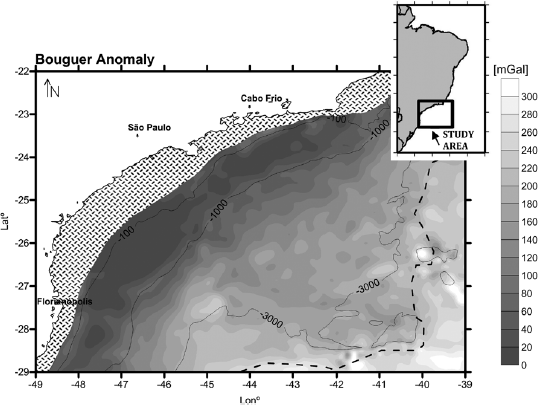
Figure 3 Bouguer anomaly from Molina (2009). The continent-ocean boundary, according to Cainelli and Moriak (1999), is represented by the dashed line and the bathymetric isolines for water depths 100, 1,000 and 3,000 m are shown. The hatched area next to the coast represents an area where the data are not reliable.
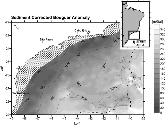
Figure 4 Sediment correct bouguer anomaly. The continent-ocean boundary, according to Cainelli and Moriak (1999), is represented by the dashed line and the bathymetric isolines for water depths 100, 1,000 and 3,000 m are shown. The hatched area next to the coast represents an area where the data are not reliable.
In addition to the cut-off wavelength and the density contrast, a reference depth value had to be assumed, and for that, several tests were performed changing the reference depth within 20 km - 35 km. For each result, the Root Mean Square Error (RMS) in relation to Moho depth values from Zalán et al. (2011) was calculated. The best RMS (0.9 km) was found for a reference depth of 31 km. The calculated Moho is shown on Figure 5.
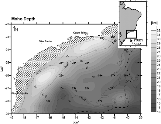
Figure 5 Moho Interface map obtained from inversion of the gravity field. values marked in black are constraining data from Zalán et al., (2011). Isolines for Moho depths of 17 km, 20 km, 23 km, 25 km and 28 km are set to reference level. The continent-ocean boundary, according to Cainelli and Moriak (1999), is represented by the dashed line and the bathymetric isolines for water depths 100, 1,000 and 3,000 m are shown. The hatched area next to the coast represents an area where the data are not reliable.
Found the Moho depth, its gravity effect was calculated by Parker algorithm (Parker, 1972) for a constant density contrast along the interface. This effect and the gravity effect of the sediments were subtracted from the observed gravity anomaly, resulting in a residual field which is associated with the basement.
For the inversion of this residual field, a constant density contrast of 1,640 kg/m3 was used, related to the density contrast between the upper crust and the water. All wavelengths are taken into account and the reference depth was defined as the zero level (Hwang, 1999). By "basement" in this study we refer to the physical surface that lies below the sediment layer. The sediment thickness data used in this study represents the depth of the acoustic basement, defined, according to Constantino & Molina (2014), as the deepest observable reflector in the seismic reflection profiles, and may not necessarily represent the base of the sediments. Furthermore the sediment isopachs are relatively smooth with respect to the gravity signal which is used to find the details of the top basement. The result of the present study work provides the base of the sediments and the results are shown on Figure 6. The values amount to 10,500 m at the central portion of the basin, near the bathymetric level of 1,000 m, coinciding with the high sediment thickness values (Figure 2).

Figure 6 Basement Depth. The continent-ocean boundary, according to Cainelli and Moriak (1999), is represented by the dashed line and the bathymetric isolines for water depths 100, 1,000 and 3,000 m are shown. The hatched area next to the coast represents an area where the data are not reliable.
Step 2 - Forward modelling
During step 2, three profiles in the Santos Basin were modelled in order to obtain the geological information and the values of the gravity field. Model 1 was built only with the horizons obtained by gravimetric inversion, where three sedimentary layers were considered: mantle, crust and sediments (Figure 7).
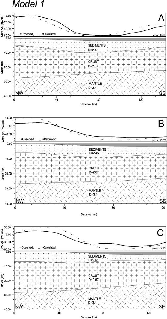
The density values used for the three profiles are average values, being 2.45 g/cm3 for the sediment layer, 2.67 g/cm3 for the crust and 3.4 g/cm3 for the mantle (Mio, 2005; Gamboa et al. 2008). The gravimetric response of the elaborate models when compared to the observed anomaly shows RMS error values considered high, being 8.483 mGal for profile A, 12,757 mGal for profile B and 13.02 mGal for the profile C (Figure 7).These results were expected, whereas the salt package present in the region was not considered in the interpretation.
Model 2, developed only for the salt package in contrast with the sediments is shown in Figure 8. The observed gravity anomaly in this case is the residual anomaly obtained in the previous model (Figure 8). The salt thickness was obtained from seismic interpretation and It has an uncertainty on the order of one hundred meters. The time-depth conversion was calculated using the classic methodology (Dobrin, 1976; Dobrin & Savit, 1988) with velocities of 1.500 m/s, 2.500 m/s and 4.000 m/s for the ocean bottom, sediments and salt, respectively.
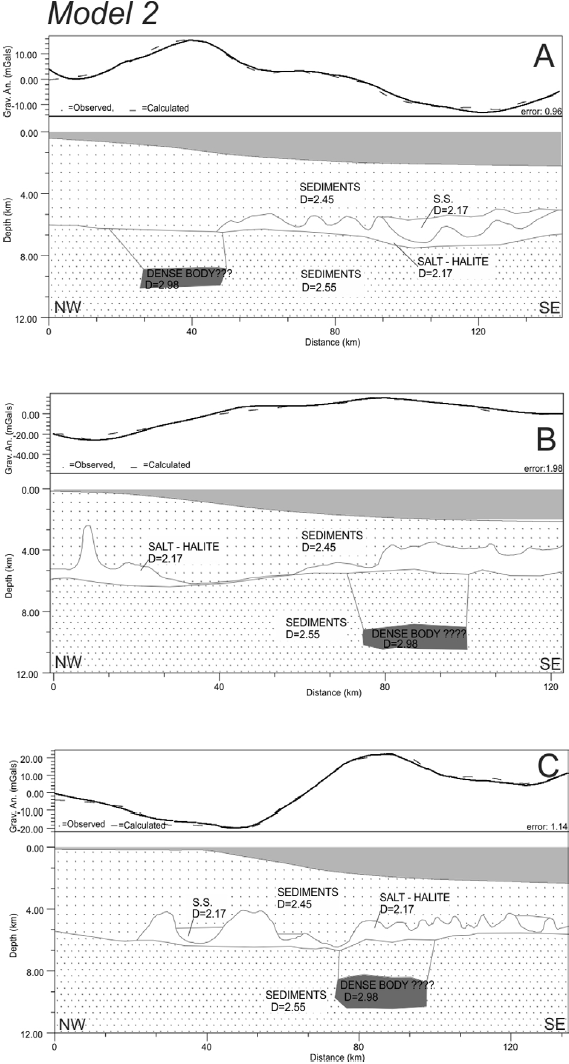
Analyzing profile A, the interpreted salt package can be observed. As the prevalence is halite a density of 2.17 g/cm3 was used. A portion of stratified salt, previously interpreted by other authors such as Cobbold et al. (2005), Mohriak & Stazamari (2012) and Mohriak et al. (2015) is also interpreted in the model. The adjustment of the observed and calculated curves in this case is satisfactory, with an RMS error of 0.96 mGal. However, in addition to the salt package, a dense body had to be added to the model.
In profile B, the presence of a dense body was also necessary and the adjustment of anomalies appear satisfactory, with an error of 1.98 mGal. The package of salt, with an average density of 2.17 g/cm3, shows a salt diapir well placed on the proximal part of the profile and a salt wall on the distal part of the profile. No evidence of stratified salt was found during the seismic and gravimetric interpretation.
The last profile also showed the presence of a dense body and a thick layer of salt, with evidences of stratified salt. The adjustment of the curves was satisfactory, with an RMS error of 1.14 mGal.
During the interpretation, the presence of anhydrite was not considered Despite having a high density compared to other sediments (2.98 g/cm3), the anhydrite when present in the salt package, appears intercalated with halite, in thicknesses that usually do not exceed 30 m, not generating a considerable response in gravity anomaly.
Discussion
Step 1 - Gravimetric inversion
The Moho values obtained by gravimetric inversion when compared to Moho values from Zalán et al. (2011) showed a RMS error of only 0.9 km. Furthermore, our model seems to be in agreement with other crust models proposed before such as by Zálan et al. (2011), Mohriak (2014) and Rigoti (2015), where they presented a very similar Moho high next to the continent-ocean transition. In the model, it is possible to see a "tongue" structure between 44-46W. This same structure is discussed by Rigoti (op. cit.) as a grabbroic proto-oceanic crust or a serpentinized mantle.
A good model of the Moho is of great importance in many geophysical and geological studies, but specially in this case, it is essential. The crust to mantle transition has the high density contrast in the Earth's upper layers, and any small changes in its depth can result in a high value of the gravity anomaly.
There are lots of studies found in the literature that make joint models of seismic and gravimetric data, but with a poor approximation of the Moho, which could result in a wrong adjustment of the observed and calculated gravity anomalies. The same happens with the basement. Because of the salt layer in Santos basin, it is very difficult to interpret what is above this layer from seismic data, and usually the basement is also an approximation. In this study, in this study, a special care has been taken with these two discontinuities, making sure that they were well delimited using the best data available for the study.
The basement structure of the Santos Basin is calculated at this last step. This is done by the inversion of the residual gravity field (gres) found in step 3, using the Iterative Gravity Inversion model (Braitenberg and Zadro, 1999). The results of this study show that some basement features, that could be determined from the available data following the methodology proposed by Braitenberg et al. (2006), are hidden by the sedimentary layer in the region of the Santos Basin.
The depth of the basement so calculated reaches 10,500 meters. Comparing to the bathymetric data (Figure 9), this depth shows greater values and it is possible to observe salient features that are not present in the bathymetric model. This can be due to the sedimentary cover that conceals some tectonic features of the basement.
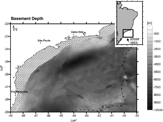
Figure 9 Bathymetric map from GEBCO. The continent-ocean boundary, according to Cainelli and Moriak (1999), is represented by the dashed line and the bathymetric isolines for water depths 100, 1,000 and 3,000 m are shown. The hatched area next to the coast represents an area where the data are not reliable.
Step 2 - Forward modelling
In this study, the initial hypothesis was that the residual anomaly obtained in the Model 1 (Figure 7) is linked to the salt package in the Santos Basin region. To confirm this hypothesis, the interpretation of the salt with this residual anomaly and the adjustment of the observed (in this case, the residual) and calculated curves was analyzed.
For profiles A and C, a layer of stratified salt was interpreted. According to Gamboa et al. (2008), the stratified salt consists of interbedded salt, such as anhydrite, halite and complex salts, deposited in shallow waters inside mini basins. Even with the possible presence of anhydrite and complex salts with higher densities than halite in the stratified salt package, we used the average density value for halite, 2.17 g/cm3, and the results can be explained by two arguments: the first one is the good adjustment of the observed and the calculated gravimetric anomalies, and the second one is due to the gravimetric method that is unable to discern this type of horizontal stratification within a larger sedimentary package.
For the three studied profiles, the presence of a dense body was pointed out and the curves were adjusted satisfactorily. To analyze it, another model was prepared (Model 3), this time with all the information presented in the results: mantle, crust, lower sediments, salt package and upper sediments (Figure 10).
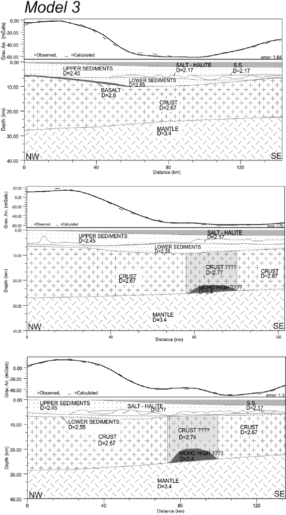
In profile A (Figure 10), the suggested dense body can be explained by a seaward-dipping reflector (SDR), which represents flood basalts rapidly extruded during the rifting or seafloor spreading. According to Jackson et al. (2000), SDRs can be present but seismically obscured bellow salt basins. After interpreting the dense body as a flood basalt, with a density of 2.8 g/cm3, the observed anomaly, when compared to the calculated anomaly, shows an error of 0.96 mGal, which can be considered very small.
To adjust the observed and the calculated anomalies of profiles B and C (Figure 10), two possible interpretations were made. The first one is a laterally density variation into the crust. For all modeled profiles, a constant density of 2.67 g/cm3 was used for the crust, because there were not enough information to assume neither a lateral density variation nor a depth variation in the lower and upper crust.
Where a dense body is modeled in both profiles B and C, the anomalies can be fitted dividing the crust vertically and changing densities from 2.67 to for 2.74 and 2.77 respectively (Figure 10).
Another possible interpretation could be a Moho high, marked in dark gray on profiles B and C (Figure-10). Some authors, such as Gomes et al. (2009), Zálan et al., (2011), Kumar et al. 2012 and Mohriak, (2014) show the presence of a Moho high in the Santos Basin, discussed in their articles as a piece of exhumed mantle. A possible explanation for the exhumed mantle would be due to the lithospheric stretching associated with crustal thinning and mantle exhumation by detachment faults. According to Zálan et al. (2011), the exhumed mantle occurs in the continental-oceanic crustal transition and can be mapped continuously from the Santos to the Espírito Santo basins. As can be observed in Figure 1, the lines are far away from the continental-oceanic crustal transition, and therefore the Moho high interpreted in our data cannot be explained by the exhumed mantle. In this case, as the Moho model is a smooth surface, this high could be explained by a feature that cannot be detected by the methodologies used in this work.
Conclusions
The Moho depth obtained from the inversion of the corrected gravity field was satisfactory and presented an RMS error of approximately 0.9 km between the values of the obtained model and constraining data from Zalán et al. (2011). The basement depth, also found from gravity inversion, could not be constrained due to the absence of previous works in the studied region. Nevertheless, during the forward modelling where the observed and calculated anomalies were compared, the use of the basement and the Moho depth resulted in a good adjustment of the gravity anomaly curves, which confirms the validity of the basement depth model.
The first forward model (Model 1), using information from the mantle, the crust and the sediments delimited by the Moho and the basement obtained by gravity inversion, showed high RMS values between the observed and calculated anomalies for all the 3 analyzed profiles. This was expected because the salt package was not considered during this first interpretation. Moreover, the main goal of this study is to associate the residual anomaly to the salt package present in the region, and the poor obtained adjustment may reflect this situation, as the salt package represents a high density contrast body that was not considered in this interpretation.
When the residual anomaly obtained from Model 1 is adjusted considering the presence of the salt package inferred from seismic data (Model 2), the errors between the observed and the calculated anomaly still remain high, and a body with high density should be added to the model in order to obtain a reasonable fit. This body could not be observed in the seismic data, probably because below the salt layer the seismic reflectors barely can be detected. Additionally, the presence of anhydrite was not considered in the model. It might appear intercalated with halite and the gravimetric method is unable to discern this type of horizontal stratification within a larger sedimentary package.
One last model (Model 3) was built with all the information obtained during this study: the upper sediments, the salt package, the lower sediments, the basement, the crust, the Moho and the mantle. The error so obtained is very low for all the 3 studied profiles. The salt package could not account for all the residual anomaly, and a possible basalt intrusion or a Moho high were suggested to explain the dense body proposed in Model 2.
As a final conclusion of this work, it is shown that the combined analysis of the two used geophysical methods can provide important information about the crustal structure and to assist in modelling the salt layer. For a future study, it would be interesting to work with an inversion method and apply it to the residual gravity anomaly. If this anomaly could be free of influences such as the basalt intrusion and the Moho high presented in this study, the inversion of the residual anomaly could be directly associated to the salt package. This could bring a new methodology where the gravity data may play a major role associated with seismic data to characterize structures containing salt packages, which could be of great interest for pre-salt studies and oil exploration.

