


 nova página do texto(beta)
 Inglês (pdf)
 Artigo em XML
 Referências do artigo
 Enviar este artigo por email
 Citado por SciELO
  Similares em
SciELO
Similares em
SciELO 
 Permalink
Introduction
Lake Chapala is the Mexico largest lake and the third largest in Latin America. It is located at approximately 20°N; 103°W, 1542 m above sea level. It measures 75 x 25 km, and has an average depth of 6 m and a maximum depth close to 11 m (Figure 1). The lake's tributaries and effluent systems are the Lerma and Santiago rivers. There is a mountain ridge along its southern and northern shores. The Lerma-Chapala watershed system has a surface area of approximately 47000 km2 (Sandoval, 1994; Aparicio, 2001). The average precipitation in this area is about 750 mm per year, which drops to 300 mm in drought years and reaches 1200 mm in wet years. The annual surface evaporation is about 1400-1600 mm, which exceeds the average precipitation by a factor of 2 (Jaurégui, 1995; Filonov et al., 1998).
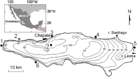
Figure 1 Bathymetric map of Lake Chapala. Depth is given in meters in relation to the 87 m isobaths. Arabic numerals sites meteorological stations are shown: 1- Jocotepec, 2 - Atequiza, 3 - Chapala, 4 - Poncitlán, 5 - Jamay, 6 - Tizapán and 7- Isla de Alacranes.
The deficit is balanced by the influx of water from the Lerma River and runoff from its basin (Mosino and Garcia, 1974; Jáuregui, 1995; Filonov and Tereshchenko, 1997). In the years of drought the annual precipitation decreases to 500 mm and there is no outflow from the lake into the Santiago river (Riehl, 1979). However, in wet years when the annual precipitation reaches 1000 mm, the river has outflow.
Local winds and breezes play a crucial role in the lake's dynamics. They develop daily, as a result of the large temperature difference between the lake's surface and the surrounding land covered with scarce vegetation. Consequently, the land becomes quickly heated and cooled during the day and night. Daytime breeze is stronger than the night time breeze and heading towards the land. During the daytime, the lake breeze speed reaches 8-10 m/s, whereby the evaporation from the lake's surface is of greater intensity than at night time (Filonov, 1998; Filonov et al., 2001).
The lake plays an essential role in the economy of Mexico. During the past decades, the lake became polluted with anthropogenic agents, which enter into the lake from the Lerma River and adjacent areas (Hansen, 1994; Hansen and Manfred van Afferden, 2001; Jay and Ford, 2001). The pollution results in the rapid growth of water lilies and Typha latifolia. Furthermore, the lake level has dropped because of the irrigation and domestic needs of cities. All this reduces its attractiveness as a recreational and tourist area, therefore, the Mexican government has taken measures to protect the dam and the lake from the negative consequences of anthropogenic actions (Filonov et al., 1998).
In the last two decades, researchers from the Department of Physics of the University of Guadalajara began to study the thermodynamic processes in the Lake Chapala using hydrodynamic modeling and the analysis of data collected with the use of up-to-date oceanographic and meteorological measurement devices. In this paper, we discuss the analysis of wind data collected over the lake, as well as the fluctuations in water temperature, currents and lake level. The main purpose of this study is to gain more understanding of the thermal and dynamic patterns of the Lake Chapala during the dry and wet seasons.
Materials and methods
One major impediment in the data collection across the study area is a great number of fishing nets deployed in the Lake Chapala. Hundreds of people are engaged in the fishing industry, which is a major source of income for them. Therefore, working there, we always rely on good luck, but do not always succeed. On some occasions, partial losses of the instruments and equipment were inevitable.
This study is based on the analysis of the temperature, currents and lake level data collected in 2005-2014 using the following oceanographic instruments: CTD SBE19-plus, SBE-39, SBE-26, HOBO V2 and a 600 kHz RDI ADCP. During that time period the measurements were not taken regularly as they pursued different goals. The sampling strategies varied with the experiment (we used different sets of instruments) and will be described in the corresponding sections.
Most measurements were taken in the deeper northern part of the lake. The meteorological data were collected from the network of seven automatic meteorological stations deployed around the lake and in its centre. The spatial structure of the temperature field and currents for the dry and wet seasons was sampled by towed temperature recorders arranged in the antenna pattern and ADCP.
Computational model
To calculate horizontal currents from wind circulation over the lake, we used the Hamburg Shelf Ocean Model (HAMSOM); a two-dimensional, non-linear, semi-implicit numerical shelf model (Backhaus, 1983). The model employs the following equations of motion:
Here U and V are zonal and southerly transports,
respectively; f = 2Ωsinφ is the Coriolis
parameter Ω = 0.04178; cycles/h is the angular velocity of the
Earth; φ is latitude; ζ is the lake level
elevation; t is time; H is water depth;
AH is the horizontal eddy
viscosity coefficient;
Results
Lake level and temperature variations at a single point
Previous studies have shown that the main processes that exert primary control over climatic conditions and water circulation in the Lake Chapala are the local winds and lake breezes (Filonov et al., 1998). The main power source of the lake breeze circulation is the diurnal temperature cycle caused by the daily variations of (a) incoming solar radiation and (b) heating of the underlying surface and to atmosphere. The interaction between the land, lake and atmosphere is a very complex system with many feedbacks. The area around the Lake Chapala is mountainous, with valleys of various spatial orientations. The thermal energy pulsates with daily periodicity but does not remain at a fixed frequency. It is redistributed at different frequencies in a complex way in the form of fluctuations (Scorer, 1978).
The lake level and temperature data in our experiment were sampled every 5 minutes by a SBE-26 temperature-depth recorder (the accuracy is 0.002 °C for temperature and 1 mm for depth), which was deployed on the mooring in the northern part of the lake, at the water depth of 2 m. The measurements were taken from 20 April to 12 September 2005 (153 days). Figure 2a shows that the seasonal level fluctuations in 2005 strongly depend on the evaporation and precipitation over the lake and its watershed. In April and May, the level dropped at a rate of about 30 cm / month, and then, until the middle of September it raised more rapidly, about 50 cm / month. In July, the level remained almost unchanged because of the reduced rainfall during this time of the year, which usually occurs over the territory of Central Mexico and is called "canicula".
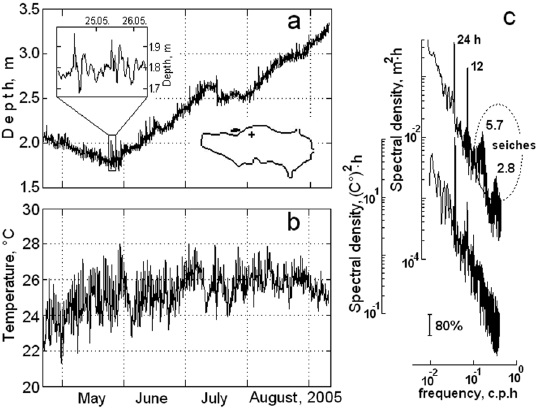
Figure 2 (a) Hourly fluctuations of lake level and (b) temperature fluctuations at a mooring during the experiment in the summer 2005. (c) Frequency spectra of a level and temperature fluctuations. Arabic numerals showing the period of the main peaks in the spectrum. The vertical line shows the 80% confidence interval.
The SBE-26 time series also shows that the daily fluctuations of lake level are determined by diurnal and semidiurnal harmonics. At a single point, the level fluctuations occur at times of the amplification and easing of the breeze whose speed was measured at the weather station Chapala (Filonov, 2002). The breeze forcing is the main source of energy for all kinds of motion in the lake. With a well-defined diurnal cycle, this breeze varies from virtually a calm at night and morning to steady northerly winds up to 6 m/s (gusting up to 10-12 m/s) in the afternoon. Since breeze circulation occurs over the entire lake throughout the year, it is expected to play an important role in the mechanisms of vertical and horizontal mixing within the lake.
The analysis shows that the start of wind intensification lags the time of the downturn of the lake level by less than two hours. The rise and drop of the level are asymmetrical. The trough lasts longer than the peak which is apparently caused by the asymmetric impact of the wind on the water surface.
As seen from the data (Figure 2b), the amplitude of the daily temperature fluctuations at the mooring site are 2-3 °C at the 2-m level and decrease to 1-1.5 °C as the instrument depth increases due to the higher lake level during the summer months.
Figure 2c shows the average spectra computed from the time series of lake level and temperature variations. The level spectrum reveals the presence of free seiche waves with 5.7 and 2.8-hour periods in the lake. Their mean square amplitudes are 15.4 and 8.1 mm, respectively. The lake is shaped like an ellipse whose axes vary in size, therefore the oscillations with a period of 5.7 hours likely correspond to the seiches propagating along the greater axis of the ellipse (west-east). The other oscillation mode is related to the seiches propagating along its smaller axis (north-south).
We used the Merian equation (Le Blond and Mysak, 1978) to evaluate the theoretical periods of the two principal waves. The period of lake-level oscillations of the first mode is given by
The principal dynamic process that occurs in the lake is the lake breeze circulation. Daytime breeze speed does not usually exceed 4 m/s. Beyond any doubt the lake breeze causes the increase in the evaporation from the lake's surface. Lake breeze, together with atmospheric pressure variations, generate free seiche waves.
North-south temperature cross-section of the lake
The spatial distribution of surface temperature across the Lake Chapala was previously discussed in the work of Tereshchenko, et al., 2002, based on extensive satellite data sets with high spatial resolution. In that study, it was shown that the northern part of the lake is warmer than its central and southern parts, which is caused by the specific features of its circulation.
To confirm this finding and shed light on other processes that occur in the lake, north-south temperature cross-sections were carried out in February, April, July and October 2006. Each survey included 60 equidistant bottom casts, 250 m apart. The SBE19-plus CTD profiler with 0.17-second sampling rate was manually dropped from the boat with a speed of about 0.1 m/s. The coordinates of the casts were fixed by the Global Position System (GPS).
The measurements were taken in the morning (from 7:00 to 9:00 am), so that the temperature along the cross-section was not biased. The cross-section extends from the northern coast (near the town of Chapala) to the south side of the lake. The spatial distribution of temperature at the cross-section is shown in Figure 3.
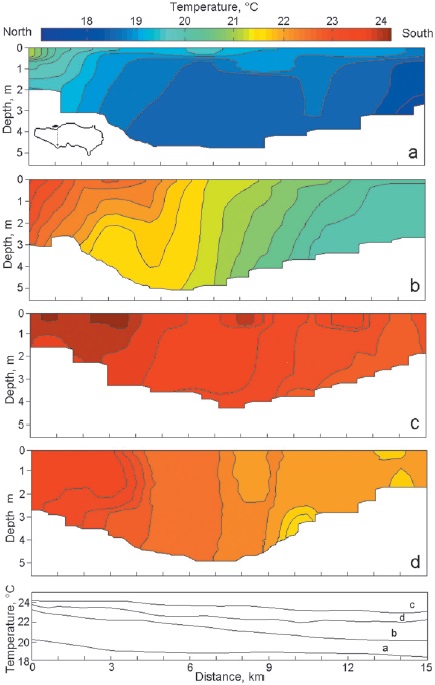
Figure 3 Vertical sections of temperature variation across the lake made in February (a), April (b), July (c) and October 2006 (d). In the lower part of the figure shows the graph of the vertical averaged temperature at the sections.
It is seen from the Figure that the in situ measurements confirm the previous finding, namely that in all seasons the temperature in the central and northern parts of the lake is higher than in the southern part. This holds true not only for the surface but also for the bottom layer. In all four seasons, vertically-averaged temperatures at the north and south ends of the cross-section differ by 2-3 °C. The vertical distributions of temperature on the sections are uneven.
The northern part of the section shows the penetration of warm water from the anticyclonic gyre which is stationary in the study area at morning time. In April, July and October, the water columns in the central and southern parts of the lake were poorly stratified, which was probably caused by vertical mixing at night time. These results shed new light on the thermal structure of the lake obtained and discussed in previously studies (Filonov and Tereshchenko, 1999a; Filonov, 2002; Tereshchenko et al., 2002; De-Anda, 2004). They should be taken into account in the design of future experiments in the study area and 3D model simulations.
Current simulations in the lake
In this study the current simulation was carried out using the HAMSOM 2-D hydrodynamic model (see appendix A) for a 30-day period during the dry and wet seasons. The model was initialized with wind fields from the network of weather stations in the Lake Chapala area collected in 2006-2007 (Figure 4). The river runoff data were obtained from CONAGUA (Mexico's National Water Council). The wet-season average of the inflow from the Lerma river was set to 600 cubic meters per second, the outflow through the Santiago river - 120 cubic meters per second.
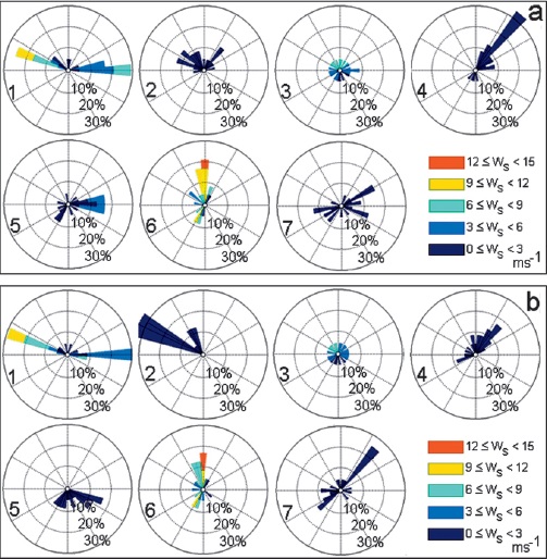
Figure 4 Annual wind rose at meteorological stations around the lake: a) for the dry season; b) for the wet season. The data was averaged for 2006-2007.
We have performed 2D model simulations for the two seasons, for which we had acquired the current data using a towed ADCP. The simulations were performed on a bathymetry grid with a 300 x 300 m spatial resolution (97 rows and 270 columns) and 3-second time step.
The model results are shown in Figure 5 as vector plots of current fields at 4-hour intervals. The breeze-induced circulation pattern in the lake is represented by two gyres. One of them is cyclonic (counterclockwise rotation) and located in the east-central part of the lake. The other gyre is anticyclonic (clockwise rotation) and located in the west-central part. The model results exhibit a very complex dynamics, whose small-scale features are difficult to interpret. Nevertheless, similar gyres were identified near the east and west coast.
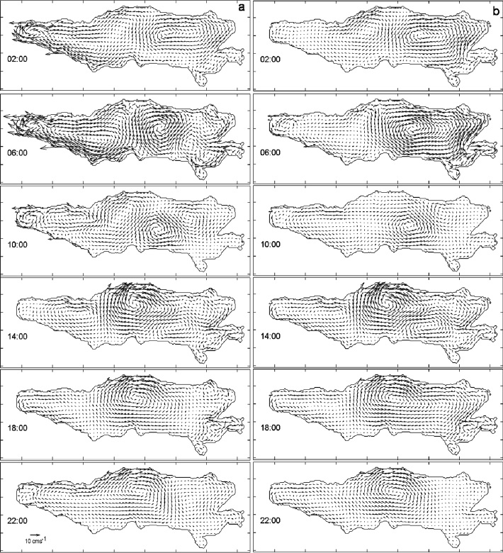
Figure 5 Result of the currents simulation induced by the wind fields in the lake: a) for the dry season; b) for the wet season. The data was averaged for 2006-2007.
The core of the anticyclonic gyre which was generated in the west part of the lake propagates to the northwest and continues to develop during the most part of the simulation period. Conversely, the cyclonic gyre originally located in the east-central part moves to the south-west part of the lake. Subsequently, it vanishes due to the bottom friction and its remainder merges into the returning flow of the anticyclonic gyre. The model simulations show that the currents near the south and north coast reach 12 cm/s. These and other model results require the comparisons with current meter data. Therefore, two special experiments were carried out in January 2007 and June 2014.
Temperature and currents variability within two lake polygons
In order to quantitatively describe the spatial-temporal variability of temperature and circulation in the Lake Chapala, two special experiments were conducted: (i) on January 10, 2007 (the Alacranes polygon, Figure 6a, center-left) and (ii) on June 1, 2014 (the Mezcala polygon, Figure 6a, center). Both experiments were conducted with the use of a vertical array of temperature recorders and a boat-mounted ADCP.
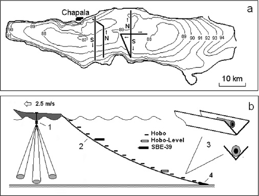
Figure 6 a) General scheme of experiments on Lake Chapala conducted on January 10, 2007 (polygon Alacranes left of the center of the figure) and June 1, 2014 (polygon Mezcala, in the center of the figure). b) Scheme of the towed sensor system. 1600 kHz RDI ADCP, 2 - Metallic angular pattern in which fixed thermographs, 3 - thermograph's mount, 4 - lattices for deep penetration of the chains.
The array contained 15 temperature recorders (13 HOBO Pro v2, one HOBO-LEVEL sensor and one SBE-39), evenly placed from the surface to 7.2-m depth. The array was towed by the boat. A down-looking ADCP RDI 600 kHz set up in bottom-track mode was mounted on the starboard side of the boat. The bin size was set to 15 cm (the total of 13 bins) and the ensemble interval was 15 sec.
The instruments were protected from fishing nets by a specially designed triangular metal case shaped to fit the recorders so that no damage was caused by the fishing gear. The designated depth of the array was controlled by HOBO-LEVEL and SBE-39 pressure sensors and weights (Figure 6b). The sampling rate of temperature and pressure sensors was 1 min. The towing speed of about 2 m/s allowed the acquisition of temperature and currents data with the horizontal spatial resolutions of 120 and 30 m respectively.
The ADCP data were processed in accordance with Trump and Marmorino (1997) and outliers were removed following the procedure described in Valle-Levinson and Atkinson (1999).
The Alacranes Polygon
The spatial distribution of temperature along the transect S (carried out from 12:00 to 14:30, the boat sailed southward) is shown in Figure 7a. The transect N (on which the boat sailed from south to north) was carried out from 16:40 to 17:50 and the corresponding temperature field is shown in Figure 7b. On both transects, the meteorological conditions were recorded. During the transect S the average air temperature was 14.5 °C; the wind was blowing onshore, and its speed was 12 m/s. Later, during the transect N, the average air temperature was higher and reached 20.9 °C; the wind was blowing offshore, which is a typical breeze circulation in the Lake Chapala (Filonov, 2002).
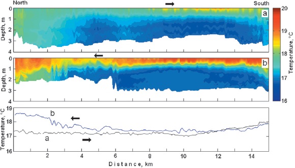
Figure 7 Vertical sections of temperature variation across the lake made on transect north-south (S) and south-north (N), registered by the sensor chains on January 10th, 2007, in Chapala's lake. The lower figure is a vertically average spatial range from the transect S and transect N.
It is seen from these transects that the heat fluxes were directed towards the surface layer of the water column, whereby the vertical gradient reached 2.5 °C per the top meter of the column. During the transect a), all temperature fluctuations were confined between 17 and 18.5 °C. A few hours later the rapid development of a thermocline was observed on transect b) (Figure 7) with temperatures ranging between 17 and 20 °C. At the end of the b) transect, the coastal water began to mix due to the lake breeze effect. Furthermore, at the north end of the transect a) the water was warmer than at the south by 1°C (Figure 7).
The wind field is believed to be the main mechanism that continually sustains the circulation in the Lake Chapala, including the gyres. Figure 8 presents the vector plots of vertically averaged currents measured by the towed ADCP and simulated by the HAMSOM model. In general, the modeled and observed data are in good agreement.
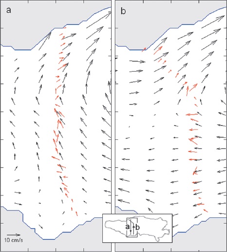
Figure 8 (a) Modeled currents (black vectors) versus currents observed (red vectors) in the area of the S transect sampling, and for N transect. The experiment was conducted on January 10, 2007, the simulations were at 12:30 and 19:00, respectively.
The transect a) was carried out from 12:00 to 14:30, while the boat was sailing from north to south. The speed of the northeastward flow along the transect peaked at 10 cm/s. The flow was presumably generated by the prevailing onshore wind dubbed "the Mexican" by local fishermen (Avalos, 2003). The 13:00 model simulations are in good agreement with the data collected in the northern part of the lake (Figure 8a). At the same time the south part is characterized with a significant difference between the modeled and observed data, both in terms the currents and temperature field.
Nevertheless, the transect b) data collected between 16:30 and 18:00 show fairly good agreement with the southern part of the 18:00 model field, with velocities reaching 15 cm/s. It was found that in the southern part of the lake, the direction of the flow can change from west to south in only two hours. The wind speed of 12 m/s was recorded by the Chapala city weather station at the same time when transect a) displayed southeastward flow. In just two hours upon the completion of transect b) the wind changed its direction to southeastward and gained speed of 10 cm/s. These results suggest that the model successfully simulates the effect of the morning breeze circulation.
The Mezcala Polygon
The model simulations show the presence of a steady anticyclonic gyre of 10-12 km diameter in the central part of the lake, across from the town of Mezcala, during both seasons (Figure 5b). To confirm these numerical calculations we have carried out the Mezcala polygon survey. The temperature and currents within the gyre where observed with the use of towed temperature recorders and ADCP. The cross-shaped polygon of about 6-km length was situated in the deepest part of the lake, inside the gyre. Continuous measurements along the three directions (Figure 6a) were taken on July 1, 2014 from 8:30 to 19:00, whereby the boat was sailing back and forth.
Presented in Figure 9 are the temperature distributions along the two transects: the transect a), which was carried out from 8:30 to 10:20, while the boat was sailing south and the transect b), which were carried out from 17:00 to 19:00. The meteorological conditions during the experiment were typical for this time of the year: the morning was calm followed by a moderate breeze in the afternoon. The towing speed was higher than on the Alacranes polygon, therefore the deepest recorder was only at a 2.2-m depth. Nevertheless, the collected data shed a new light on the horizontal and vertical structure of the temperature field on the polygon in the presence of the anticyclonic gyre.
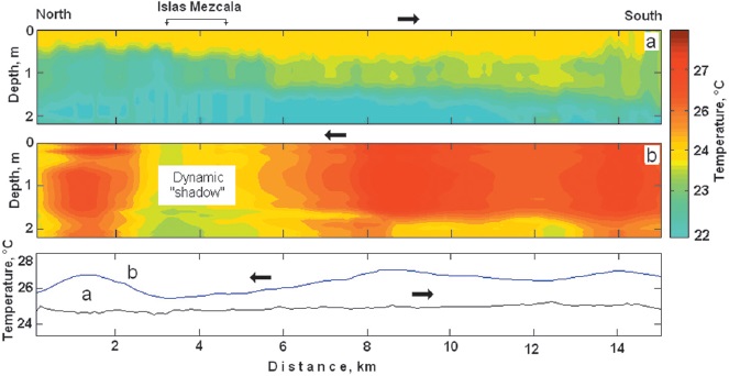
Figure 9 Vertical sections of temperature variation across the lake were taken on transect north-south (S) and south-north (N), registered by the sensor chains on July 1, 2014. (c) Vertical average spatial range from transect S and transect N. (d) Simulation corresponding to 18:00 (black vectors) versus currents observed (red vectors) in the area of sampling at polygon Mezcala.
As seen from Figure 9a, in the morning, at the time when the boat was sailing south (from 9:15 to 10:22 AM), the stratification of the lake was moderate. The average temperature near the southern shore of the lake was steady at 23.4 °C (Figure 9b). During the reverse leg along the transect (from the south to the north) the measurements were taken only in the afternoon (from 17:00 to 19:00), when the wind and temperature conditions over the lake were quite different from the morning. The simulated currents are reasonably comparable with the observed data and suggest that in the second half of the day the gyre was well-developed. The gyre exerts a strong impact on the spatial temperature distribution in the study area.
A zone of strong vertical mixing was discovered on the last leg, about 1 kilometer east from the Mezcala Islands, when the array of the recorders was towed from the south to the north. These islands are about 1.5km long. They are perpendicular to the flow of the gyre and create dynamic shadows (the shaded area in Figure 10). Within this area, the upwelling of cold bottom water due to the Bernoulli effect resulted in its mixing with the warm surface water. Unfortunately, the spatial grid of the model (300x300 m) was too coarse to simulate this effect.
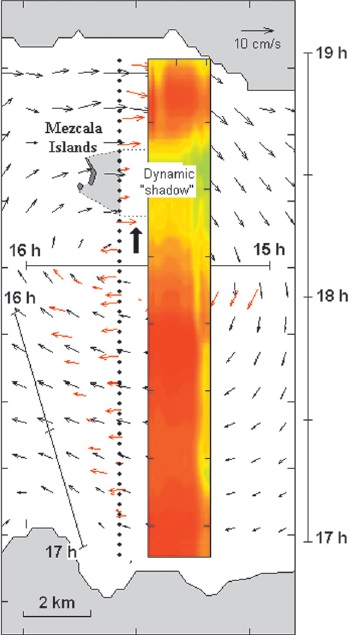
Figure 10 Modeled currents (black vectors) versus currents observed by towing ADCP (red vectors) at the Mezcala region. The experiment was conducted on January 10, 2007. The simulations were from 15:00 to 19:00, respectively. The bullet points with the arrow show the direction of the towed sensor system on the section of South-North. Color stripes are a sectional view of the temperature field. The straight thin lines on figure show the sections taken at appropriate times.
More detailed hydrographic surveys off the Mezcala Islands and the Alacranes polygon are planned for the future with the subsequent assimilation of the collected data into 3D numerical models. This will allow us to confirm the above mentioned assumptions about the impact of the vortex on the vertical and horizontal mixing near the islands.
Discussion and conclusions
A great deal of results presented here are unique for the Lake Chapala. Although this study was carried out during different time periods, on average it gives a fair account of the dynamic processes occurring in the lake and its surroundings. The main dynamic process occurring in the lake is the breeze circulation. The daytime breeze does not usually exceed 4 m/s. Beyond any doubt the lake breeze results in the increased evaporation from the lake's surface and also generates free seiches waves.
The spectral analysis of the lake level fluctuations measured by a high-precision HOBO-Level recorder shows that there are two seiches modes in the lake with the periods of 5.7 and 2.8 hours, with the average amplitudes of 15.4 and 8.1 mm. Our earlier study (Filonov, 2002) reports almost similar results, except that there is no well-defined mode with the 2.8-hour period due to the weak amplitude. The seiches generate periodic currents which peak at 1 cm/s in nodal line areas (Filonov, 2002).
The spatial distribution of surface temperature in the Chapala Lake has been previously discussed in the works of Filonov and Tereshchenko, 1999a, 1999b; Filonov et al., 2001; Filonov, 2002, based on the data sets acquired with the use of high-precision instruments. Tereshchenko, et al., 2002 report the results of the analysis of fairly long temperature data sets remotely sensed with high spatial resolution (the AVHRR-NOAA satellite images). The study shows that the northern part of the lake is warmer than its central and southern parts, which is essentially an important feature of the circulation. However, until now there were no detailed accounts of the horizontal and vertical structure of the temperature field in the lake in different seasons.
Our in situ measurements taken in February, April, July and October 2006 confirmed the previous finding that the temperature in the central and northern parts of the lake during different seasons is always higher than in the southern part, which holds true not only for the surface but also for the entire water column. In all four seasons the average temperatures at the north and south coast's differ by 2-3 °C. The vertical distribution of temperature along the transects was not homogeneous.
The results of numerical simulations of the Lake Chapala circulations are reported in some publications (Simons, 1984; Escalante, 1992; Filonov and Tereshchenko, 1999a; Filonov, 2002; Avalos, 2003), but none of them is based on the experimental and observational wind data sets collected in the study area during different seasons.
In this study the simulation of currents was carried out by means of the 2D HAMSOM model for the dry and wet seasons. The model was initialized with the wind data from the network of weather stations in the Chapala Lake area collected in 2006-2007. The model results demonstrate very complex dynamics, in particular, the continuous presence of two gyres. One of them rotates counterclockwise (cyclonic rotation) and is located in the east-central part of the lake. The other one rotates clockwise (anticyclonic rotation) and is located in the west-central part.
In order to describe the spatial-temporal variability of temperature in the lake and compare the model simulations with the observed data, two special experiments were conducted in the Lake Chapala on January 10, 2007 (polygon Alacranes) and on June 1, 2014 (polygon Mezcala). In these experiments a vertical array of temperature recorders aligned in the antenna-like pattern was towed along the transect by a boat with onboard ADCP. These high-frequency measurements on both polygons shed new light on the distribution of temperature and currents in these parts of the lake. The data collected on the Mezcala polygon confirm the presence of an anticyclonic gyre and show the influence of the islands on the dynamics of water masses and the temperature distribution in the lake.

