


 nueva página del texto (beta)
 Inglés (pdf)
 Artículo en XML
 Referencias del artículo
 Enviar artículo por email
 Citado por SciELO
  Similares en
SciELO
Similares en
SciELO 
 Permalink
Introduction
Mandelbrot (1967) developed the fractal geometry that allows describing scale invariant phenomena. That is, the spatial variation of a fractal parameter often looks similar at a wide range of scales. Examples in Earth Sciences range from the geological type (e.g., rocky coast line, faulting, seismicity, volcanic eruptions) to the geophysical information such as gravity and magnetic field data, topography, among others.
The fractal nature of a variable is evident from the fact that the power spectrum P (k) is proportional to kb where k is spatial frequency and b is the scaling exponent that is in practical terms, for instance, the slope of the spectrum in a log-log space. For gravity data, β values range from -3.8 to -5 based on regional or global studies (Maus and Dimri, 1994; Chapin, 1996; Pilkington and Todoeschuck, 2004; Dimri, 2005; Pilkington and Keating, 2012). Among other applications, the fractal structure of gravity or geomagnetic information has been used in computing the optimum gridding interval (Keating, 1993; Pilkington and Keating, 2012), depth estimation (e.g., Pilkington and Todoeschuck, 2004; Gregotski et al. 1991; Maus and Dimri, 1996; Quarta et al. 2000), inversion of potential field data (Pilkington and Todoeschuck, 1993), determining the optimal Bouguer density to be used for topography reduction of gravity data (Thorarinsson and Magnusson, 1990; Chapin, 1996; Caratori Tontini et al., 2007).
Chapin (1996) computed an isostatic residual gravity map for South America based on both the fractal nature and correlation of regional gravity anomalies and topography. The use of these maps in exploration is widespread because they would clearly depict the distribution of densities in the upper part of the crust (Simpson et al., 1986; Jachens et al., 1996). However, the magnitude of these residual gravity anomalies is dependent on the assumed density values for terrain, lower crust and upper mantle. In his work, Chapin (1996) estimated the optimum density of topography by analyzing the changes in fractal dimension (D) of simple Bouguer anomalies (without terrain correction) calculated with varying densities. As a result, he found a minimum curve superimposed on a regional trend when plotting the curve of fractal dimension versus density. In contrast, Thorarinsson and Magnusson (1990) for Iceland gravity data and later Caratori Tontini et al. (2007) for a Mediterranean Sea gravity database, determined simple minimum D versus density curves (U-shaped). This particular feature of D versus density curve for South American data has been attributed to either a long wavelength component (Chapin, 1996) or the use of simple Bouguer anomalies (slab formula reduction), neglecting terrain corrections (Caratori Tontini et al., 2007).
Herein, we investigate the fractal nature of onshore gravity anomalies for Chile, Argentina and part of Uruguay, and present a new map of isostatic residual anomalies. Unlike Chapin (1996), who used the power spectral method, the fractal dimension estimation is carried out using the variogram technique for the terraincorrected Bouguer anomalies. For this study, a more detailed gravity database, which provides a better resolution in regions such as Chile and some Argentine sedimentary basins, was available.
Topographic and gravity database
The study area ranges from 21° S to 55° S in latitude and 75° W to 55° W in longitude. The gravity database is part of the South American Gravity Project (SAGP) and the Anglo Brazilian Gravity Project (ABGP), carried out under the umbrella of the International Association of Geodesy (Pacino, 2007). The gravity data points were provided by different sources: national and international academic institutions, oil and mining companies and the Geographic National Institute of Argentina (IGN). The data were homogenized and linked to the IGSN 71 gravity datum and referred to the Geodetic Reference System 1980 (GRS80). Data errors are assumed to be less than 0.5 x 10⁻⁵ m/s2 (0.5 mGal). The dataset of the land free-air gravity anomalies is depicted in Figure 1.
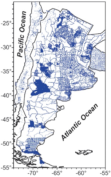
Figure 1 Geographical distribution of free air gravity anomalies data over the studied area (point station in blue).
The topographic data used for gravity terrain reductions calculations are based on the SRTM_30 PLUS digital elevation model data (Becker et al., 2009).
Fractal dimension of gravity anomalies and topography
The fractal dimension of gravity anomalies has been estimated using spectral methods (Chapin, 1996; Caratori Tontini et al., 2007) or variogram techniques (Maus, 1999; Thorarinsson and Magnusson, 1990). Maus (1999) pointed out that the advantage of using this last approach is that it avoids the distortion and loss of information inherent to the computation of Fourier-domain spectra. Thus, variograms in the spatial domain replace spectra in the transformed domain.
According to Thorarinsson and Magnusson (1990), the fractal dimension of gravitational surfaces can be estimated using a method based on the variogram of a surface whose expected value E is given by:
where Zp and Zq are values of the surface at points p and q, Dpq is the horizontal distance between points, k is a constant and H is a parameter in the range of 0 to 1, which is related to the fractal dimension D as H= 3-D. These kind of surfaces are used as a method of simulating topographic surfaces (Goodchild and Mark, 1987).
Making log-log plots of the variances of surface relief differences versus distances between points, results in a straight line over some range on which the physical phenomenon is fractal. The slope (b) of the plot is proportional to the fractal dimension for that range:
It is important to note that the fractal dimension of a data set (e.g., topography) is a number which acquires meaning when compared with the fractal dimension of another variable (e.g., gravity anomalies), obtained using the same method (Chapin 1996). In this context, the fractal dimensions for gravity anomalies and topography here determined are not directly comparables with those calculated by Chapin (1996) who used a spectral approach.
Figure 2a shows the variogram of topography data from the continental Argentina, Chile and western Uruguay database (see station points in Figure 1). The best linear trend shows a fractal dimension of 2.479 ± 0.007 for all distances, according to the recognized fractal nature of topography (Turcotte, 1997). Deviation from linearity is observed at the longest distances because of the small number of pair points.
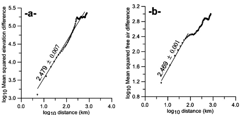
Figure 2 a) Variogram of the topography data over the study area (R2= 0,97). b) Variogram of free air gravity anomaly data set for the Chile, Argentina and western Uruguay (R2= 0,99). An estimate of the fractal dimension D is derived from the slope of the linear range of these plots. Note that fractal dimensions for topography and free air gravity anomalies are very close to each other. This demonstrates the relationship between topography and free air anomalies at wavelengths shorter than 80 km.
It has been pointed out (Chapin, 1996) that gravity anomalies are a combination of two components: one related to the topography, which is scale-independent (or fractal), and a second one, which is scale-dependent, due to the distributions of density. For instance, in the case of regions where isostatic balance prevails, the long wavelength free air anomalies are scale-dependent while the short wavelength free air anomalies show a fractal nature. Figure 2b displays the variogram plot for the free air gravity data of the studied area. Note that the data fall on a straight line between approximately 5 km and ~80 km indicating a fractal surface (D= 2.469 ± 0.001). Thus, in this range the fractal dimension of free air anomalies are nearly the same as that for topography (Figure 2a). At larger distances (> 80 km) the linearity disappears suggesting a non-fractal behavior and thus the topographic load must be supported by isostatic compensation.
Determining the optimum Bouguer density
The central idea of the fractal method to estimate a Bouguer density is based on the classical Nettleton's technique (Nettleton, 1939): the optimum Bouguer density should reduce in short wavelengths the correlation between free air gravity anomalies and be represented in the first (on the left) part of the variogram (Figure 2b) where the gravity anomalies are scale independent and its fractal dimension could be used to estimate a topographic density (Thorarinsson and Magnusson, 1990). Amongst all reasonable topographic densities, we should find the one that reduces the roughness of the Bouguer anomaly data. Minimizing the roughness of a surface is equivalent to reducing the fractal dimension of that surface.
Thus, variograms were computed for the complete Bouguer anomalies calculated for topographic densities ranging from 0 through 4000 kg/m2. Terrain reductions were calculated using the detailed digital elevation model SRTM_30 PLUS (Becker et al., 2009) and a combination of the methods described by Nagy (1966) and Kane (1962). A simple Bouguer correction by a spherical cap, computed to a radial distance of 166.7 km, was also applied. Fractal dimensions, in a range of 2.469 to 2.425, were estimated from 12 km to the distance class of 80 km.
Figure 3b depicts a plot of the fractal dimensions versus the corresponding reduction density. It results in a parabolic or U-shaped curve. A least square fit gives the optimal density value ∼2300 kg/m3 This optimum density for continental Argentina-Chile and part of Uruguay is lower than the value of 2600 kg/m3 estimated by Chapin (1996) for all South America. In our case, we use an improved database, a terrain corrected Bouguer anomalies data set and a different methodology for estimating the fractal dimension.
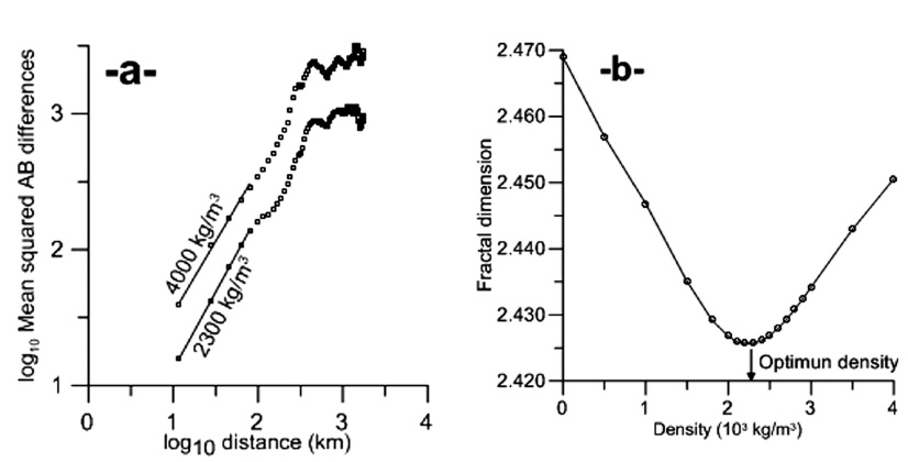
Figure 3 a) Variograms of the complete Bouguer anomalies computed for two selected densities for continental Argentina, Chile and western Uruguay. The straight segment in each curve shows the distance range from 12 km to 80 km that has been used to calculate the fractal exponent. The fractal dimensions are 2.450 and 2.425 for densities 4000 kg/m3 and 2300 kg/m3, respectively. b) Plot of fractal dimension versus density. The U-shaped curve shows a minimum at 2300 kg/m3, that is the best density to minimize the gravity effect of topography.
Map of isostatic residual gravity
Figure 4 shows the map of isostatic residual anomalies for Chile, Argentina, and part of Uruguay. The isostatic crustal thicknesses (M) in the Heiskanen-Airy system were sized from the topography (H) as follows (Simpson et al., 1986):
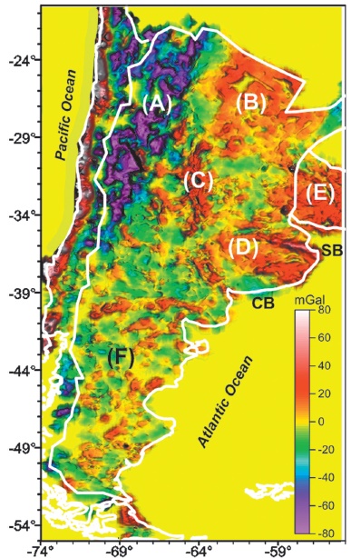
Figure 4 Map of onshore isostatic residual gravity of Chile, Argentina and western Uruguay based on an Airy-Heiskanen model of local compensation with parameters: density of topographic load 2300 kg/m3; density contrast across bottom of root, 400 kg/m3; thickness of reference crust, 36 km. Labels identifying the main isostatic residual anomalies zones (A)-(F) are shown. CB: Claromecó Basin, SB: Salado Basin. International boundaries are shown in white line.
where σt = 2300 kg/m3 is the fractal derived Bouguer density, σc = 2900 kg/m3 is the lower crust density, σm = 3300 kg/m3 is the upper mantle density and T= 36 km is the reference crust (Fromm et al., 2004). A crust-mantle density contrast of 400 kg/m3 is typically assumed at these latitudes (e.g., Introcaso et al., 1992). The gravity effect of the isostatic crust-mantle interface was calculated by the Parker's method (Parker, 1972). Then, it was subtracted from the terrain corrected Bouguer anomalies (σt = 2300 kg/m3) and thus, the resulting anomaly in Figure 4 serves as a residual field. Our results are consistent with previous residual isostatic maps carried out for this region (e.g., Schmidt and Götze, 2006).
On this map (Figure 4) some main residual anomaly patterns are recognized. In the following, they are interpreted in terms of their wavelength. Thus, long wavelength (regional) anomalies are mainly related to isostatic effects (for instance, crust-mantle interface density variations) while short (local) wavelength anomalies are attributed to geologic bodies in the middle or upper crust, which can be associated with surface or near surface geology and justified by deviations of the actual rock density from the constant topographic density here considered (σt = 2300 kg/m3). The aim of this qualitative interpretation is to explain the isostatic residual gravity field in a very general way, thus providing a basis for further geological o tectonic investigations. The anomalies are labelled (A) to (F) in Figure 4.
In the region identified as (A) on the western side of the map in Figure 4, there is a predominance of negative isostatic anomalies over the Cordillera de Los Andes, that would indicate a slight unbalance. Positive anomalies westwards would be linked to both the high density of the oceanic subducting Nazca plate that lies close to the surface and the intermediate-to-basic igneous rocks outcropping along the Andean Coastal Cordillera of Chile (Tassara et al., 2006; Prezzi and Götze, 2009).
The broad isostatic residual gravity high (B) centered over the Chaco-Paranaense basin probably does match a slightly thinned crust consistent with results from studies of seismic refraction, receiver function and surface waves (Assumpção et al., 2013).
Positive values (C) in the region of the Eastern Pampean Ranges is interpreted in relation with unbalanced isostatic state at crustal level. This Range, despite their topographic expression, has a no pronounced crustal root (Miranda e Introcaso, 1999). This result is supported by seismological studies of receiver function for local (Perarnau et al., 2012) and teleseismic events (Gans et al., 2011), who found out thicknesses of ∼35-40 km for a relatively flat Moho.
Positive residual isostatic anomalies (D) occur mainly over the Rio de La Plata Craton in Argentina which are interpreted in relation to the Precambrian metamorphic basement (i.e., Dalla Salda, 1999). A positive anomaly with approximate ONO course highlights over the Salado basin on the northeast flank of the Buenos Aires Province. This anomaly has been associated either excess of crustal thinning (isostatic unbalance) or a combination of crustal thinning and positive density contrasts attributed to the intrusive basalts present in the subsurface of the basin (Crovetto et al., 2007). Furthermore, a negative residual anomaly is observed to the southward of Buenos Aires, on the Claromecó basin. Gravimetric studies have shown that this basin exhibits crustal thinning with isostatic balance (Ruiz and Introcaso, 2011). Thus, the negative residual isostatic anomaly is related to the powerful infilling sediments (Tankard et al., 1995).
Positive residual anomalies (E) on the southwest of Uruguay would be due to the metamorphic basement of the Piedra Alta terrane (Sánchez Bettucci et al. , 2010). The association of residual isostatic anomalies with the structural features of the basement of Uruguay has already been pointed out by Oyhantçabal et al. (2011), although using different crustal parameters.
In the southern region (F), where gravity data are more sparse, it has not been possible to identify anomalies associated with geological or tectonic features.
Conclusions
The fractalness of onshore gravity anomalies for Argentina, Chile and part of Uruguay is analyzed using an updated gravity database. The fractal dimensions of topography and gravity anomaly data were estimated in the spatial domain by means of the variogram technique. Our results point out that for distances up to 80 km: 1- free air anomalies for this region are scale independent (D= 2,469 ± 0,001) and correlate well with the topography, 2- fractal dimensions of the complete Bouguer anomalies in the range of wavelength from 12 km to 80 km, were calculated by using different (t densities. The fractal dimension versus density curve shows a parabolic trend with a minimum at a density of (t = 2300 kg/m3. This density would minimize the effects of topography and therefore, it would be the optimum density to compute the complete Bouguer anomalies for the study area.
3- This ideal density was used to prepare a new isostatic residual anomaly map (Figure 4) for this region applying the concept of Airy-Heiskanen isostasy. Generally speaking, the Airy isostatic roots lead to a high-degree of compensation, but the residuals show deviations ranging ± 80 mGal. An intriguing feature on this map is that the mean level of isostatic gravity anomaly is negative. This long wavelength anomaly could be attributed to the mantle. We proceed with a general interpretation of some interesting anomalies. A regional minimum (A) along the southern Andes and a high (C) over the Eastern Pampean Ranges, both do reflect isostatic disequilibrium in a region characterized by its active tectonic. Other positive isostatic residual anomalies such as along Coastal Cordillera of Chile, the Piedra Alta terrane of Uruguay (E) and the Rio de La Plata craton (D), can be attributed to geological bodies near the surface. South of 40° S latitude, mainly less positive anomalies in patches of short wavelengths can be seen.

