Original paper

 

The intersective Hough transform for geophysical applications

 

F. Alejandro Nava

 

Seismology Dept., CICESE, Carr.Tijuana-Ensenada 3918, Ensenada, B.C., 22860, México, Tel: 52-646-1750500 x26519, Fax: 52-646-1750559. Corresponding author: fnava@cicese.mx

 

Received: September 09, 2013.
Accepted: October 15, 2013.
Published on line: July 01, 2014.

 

Resumen

La transformada de Hough es una herramienta ampliamente utilizada para identificación de alineamientos, pero el método de votación utilizado usualmente en esta transformada presenta serios problemas cuando las alineaciones no son exactas. Proponemos un método de votación basado directamente en intersecciones en el espacio de Hough, que es más eficiente y soluciona los problemas mencionados; el método propuesto también da un método directo para cuantificar cada alineamiento. El método intersectivo puede obviar el uso de espacios de Hough divididos en celdas acumuladoras, y trabajar directamente sobre cúmulos de intersecciones, de manera que todo el proceso de identificación de alineamientos puede ser automatizado. Un ejemplo sintético que representa una aplicación geofísica de la transformada de Hough, identificación de alineamientos inexactos en presencia de ruido, es usado para ilustrar el método propuesto y para discutir otras aplicaciones. Un metodo opcional de ponderación de los datos puede ser usado para tomar en cuenta posibles incertidumbres en éstos. Tanto para alineamientos exactos como inexactos, el método intersectivo da mejores resultados que el método tradicional

Palabras clave: transformada de Hough, identificación de alineamientos, alineamientos geofísicos.

 

Abstract

The Hough transform is a widely used tool for alignment identification, but the voting scheme usually used in this transform presents serious problems when alignments are not exact. We propose a voting scheme based directly on intersections in Hough space, which is more efficient and solves the above mentioned problems; the proposed scheme also provides a straightforward way of quantifying each alignment. The intersective approach can even dispense with gridded Hough spaces and accumulator cells, through direct clustering of intersections, so that the whole alignment identification process can be done automatically. A synthetic example representing a geophysical application of the Hough transform, identification of inexact alignments in the presence of noise, is used to illustrate the proposed method and to discuss further applications. An optional data-weighting scheme takes into account possible uncertainties in the data. For both exact and inexact alignments, the intersective method yields better results than the traditional one.

Keywords: Hough transform; alignment identification, geophysical alignments.

 

Introduction

The Hough Transform is a widely used tool in many applications ranging from detection and analysis of alignments in point distributions to image analysis and computer vision (e.g. Illingworth and Kitler, 1988; Hart,2009; Shapiro and Stockman, 2001; Wikipedia, 2012). Originally meant to detect alignments of points or objects along straight lines (Hough, 1959), it has been extended to detect other kinds of alignments (Duda and Hart, 1972; Ballard, 1981); we will restrict our treatment to detection of straight lines.

The usual, or traditional, Hough Transform (HT) (Hough, 1959) determines the presence of alignments of points in the physical, or observational, space, based on "votes" cast by each point onto accumulator cells in the Hough space (this process will be reviewed below). However, this voting scheme presents serious problems when the alignments are not perfect, and results in confusing Hough space diagrams when a large number of alignments is being considered.

For many geophysical applications, such as identifying alignments in earthquake epicentral (or hypocentral section) distributions, the main problem with the HT is that events are not perfectly aligned. Misalignments can occur because of location errors, but the main source of misalignment is that geophysical alignments do not occur along perfect zero-width straight lines. Hence, their curves in Hough space do not intersect at one point, and their intersections are spread over some region.

O'Gorman and Clowes (1976) proposed a method which uses the local gradient direction of image intensity to approximate the angles of lines, but this approach is appropriate for lines consisting of neighboring pixels and is not appropriate for sparsely populated alignments, like most in geophysical applications.

Fernandes and Oliveira (2008) improve the voting scheme by looking for clusters of approximately collinear points (or pixels) in observational space and casting votes using a Gaussian elliptical kernel oriented according to the direction of the line that best fits each cluster. This method is complicated because it carries out the search for lines largely in observational space. Other methods for im-proving the Hough transform are found in Kiryati et al. (1991), Li et al. (1986), and Furukawa and Shinagawa (2003).

We propose a new straightforward voting scheme which can be used to obtain much cleaner and easy to use accumulations in Hough space, or to dispense altogether with accumulator cells.

 

The traditional Hough transform

Here, we will briefly review some basic concepts of the HT, mainly to introduce our notation and to define terms that will be repeatedly used, as well as to point out characteristics of the usual HT that will be improved by our proposed approach.

The HT, as proposed by P.Hough (1959), is based on the representation of straight lines occurring in physical 2D (x, y) space by points in a 2D parameter space, the Hough space. The parameterization most commonly used is that proposed by Duda and Hart (1972), which represents each straight line in the physical space by a point in the (θ, r) Hough space, where r is the shortest distance from the origin to the line (measured along the r line, which is a straight line perpendicular to the original one and passing through the (x, y) origin), and θ is the angle between the r line and the X axis (Figure 1). The usual ranges of these parameters are 0 ≤ θ ≤ π and -∞ < r < ∞ , where r is considered negative if the line passes below the origin.

The (θ, r) parameters are related to the a and m parameters of the usual y=a+mx representation by

The line y = a + mx goes through the point (0, a) and makes an angle a with the X axis; perpendicular to this line and passing through the origin is a line with length r which makes an angle q with the X axis.

A point (x_i , y_i) in the X, Y plane can be considered as the locus through which pass an infinite number of straight lines, each characterized by an angle θ and a distance r, according to

and this family of lines corresponds to points along the curve defined by equation (3) in the Hough (θ, r) space.

For two points, (x_i , y_i) and (x_j, y_j), there is only one line common to both, and hence only one common point where the two corresponding curves in the Hough (θ, r) space intersect. For any number of points, in the physical space, their (θ, r) curves intersect at as many points as there are pairs of (x, y) points, but all points along a straight line will intersect at the same (θ, r) point. Thus, significant straight alignments, i.e. those with many aligned elements, are identified as points in the space where many curves intersect.

The traditional HT then identifies the alignments using the following scheme. The (θ, r) plane is discretized into "accumulator" cells each of Δθ x Δr size, and each (x_i , y_i) point "votes" through its corresponding curve (3) increasing by one the content of each cell traversed by the curve. Finally, cells with large values (where large numbers of curves coincide) are chosen, either numerically or visually from a color-coded representation, as representing straight lines corresponding to alignments in physical space. The number of votes in a cell, which we will denote by q, is a measure of the number of points in the line defined by the cell parameters.

This traditional scheme works well when alignments are perfect, but when alignments are not perfect, as in most cases dealing with geophysical data, the accumulator cell map is distorted, so that it may be impossible to get a sufficiently accurate identification. We will now present an illustration of the problem and discuss its general causes.

To illustrate this point, let us consider a set of 60 points (which could represent epicenters or other geophysical features) distributed over the plane shown in Figure 2 as:

•Line 1: 9 events along y = 0.300 + 0.900x (at random x values), corresponding to point θ_L1 =131.987°, r_L1 = 0.223 km in Hough space,

•Line 2: 9 events along y = 0.700 - 0.400x (at random x values), corresponding to point θ_L2 = 68.199°, r_L2 = 0.650 km,

•42 events distributed randomly with uniform probability over the plane.

The random events, more than twice the aligned ones, representing noise were included in order to have a distribution in which alignments would not be obvious, and could test the capabilities of each method. Noise is always present in geophysical observations, and the example distribution can very well represent a typical case of epicentral distribution.

The HT of this set, using cells Δθ = 1.5º by Δr = 0.015 km, is shown in Figure 3. The brighter cells correctly identify the two lines, although none of them attained the expected q=9 incidences, due to the actual location of the cells and to numerical approximations (seven decimal places in x and y); the maximum corresponding to Line 2 is spread over several neighboring cells. The identified lines are Line 1: θ_L1 = 132.000°, r_L1 = 0.208 km, y = 0.208+0.900x, and Line 2: θ_L2 = 69.000°, r_L2 = 0.643 km, y = 0.689-0.384x. Thus, we see that the HT works reasonably well for a set of points including some "perfect" alignments, although the precision is always limited by the size of the cells.

Now let us slightly distort the alignment by adding Gaussian variations from exact alignment, having zero mean and standard deviation 0.02 km, to the points in both lines (Figure 4). The sizes of the symbols are proportional to optional weights discussed later. It should be noted that small departures from alignment can cause, for points that are close together, large changes in the angle of the line through them that result in intersections that locate far from the other intersections of the line; however, for distant points the angle does not change very much and intersections locate close to the location of the original line.

The HT, shown in Figure 5, is now quite complicated, there are more cells with relatively high q, but the maximal numbers have decreased. The overall difference between high and low values is less than it should be. There are now many candidates for alignments, and the transform is incapable of distinguishing which are the high values which correspond to true, but noisy, alignments.The problem, of course, is that curves corresponding to points along a given line, but not exactly on it, do not intersect at a single point, and some of these curves may cross in different cells, which complicates the inherent ambiguity in using cells. When intersection points are located near the border(s) of a cell, they will be distributed among several cells, so the HT results depend on the actual location of the cells. If larger cells are used, to ensure that all intersections fall within the same cell, this results in less precise results, since parameter values can only be determined within ±Δθ/2 and ±Δθ/2. If smaller cells are used, the probability of having one alignment spread over several cells increases, and, most important, large values in neighboring cells cannot be used to determine the correct parameter values, because of the main flaw in the voting method of the HT: the HT cannot distinguish between lines that cross within a given cell and lines that just pass through it.

For the HT voting method, if q lines intersect within a given cell, a minimum of 2q incidences will occur within the 8 surrounding cells (for typical curvatures); in fact since (3) can be written as r = a sin(θ + β), where α= √x²_i+y²_i and β = arctan (x_i / y_i), the absolute value of its slope cannot be larger that a, so that for points distributed all over the physical space most of these 2q+ incidences will occur within neighboring cells having the same r value. The resulting high values, which correspond to non-intersecting lines, cannot be distinguished, a priori, from those from intersecting lines. If one tries to determine where the intersections should be by averaging over neighboring cells, the average will include both intersections and simple traversals, and is essentially meaningless.

Thus, it is clear that for non-exact alignments, like those associated with geophysical observations, a new voting method is needed.

 

The Intersective Hough Transform

Intersective voting

Since we are interested in the intersections of the (θ, r) curves, not on the curves themselves, we propose voting directly with the curve intersections. This we will call the Intersective Hough Transform (IHT)

From equation (3), the cosenoids for points (x_i , y_i) and (x_j , y_j) intersect at θ_ij such that

x_i cos (θ_ij) + y_i sin (θ_ij)= x_j cos (θ_ij )+ y_j sin(θ_ij)

so that

and the corresponding is given by

We will vote by increasing the value only for cells within which fall the intersection coordinates (θ_ij , r_ij).

Figure 6 shows the accumulator cells from intersective voting for the same point set of Figure 2, using, for illustration purposes, the same cell sizes as for the HT (as will be explained below, the IHT works better with cells much smaller than those for the HT). Note that there are only two cells with large values, and a comparison with Figure 3 shows how much clearer straight-line identification is with the IHT. Also, the quantification of the alignments is much more reliable and straightforward, since there is no noise from lines that do not correspond to intersections.

Voting with intersections also results in much better definition of cells corresponding to lines, because an alignment of p points, which results in q ≤ p HT votes (q = p only if the alignment is perfect and all curves cross within the same cell), will result in q ≤ p (p-1) / 2 IHT votes, a number which grows very fast compared to p for p > 3; compare the q (color) scales in Figures 3 and 6.

It is for noisy data that the IHT proves even more advantageous, because it allows better definition by using smaller cells. After a run with large cells to identify the approximate location intersection clusters for each alignment, much smaller cells can be used; then intersections will be spread among many cells as shown in Figures 7 and 8, but this is now no problem, since these cells can be combined to correctly identify the alignment.

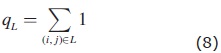
Let q_mn be the number of intersections falling in the cell located in column m and row n, and let L be the set of indices of a group of (neighboring) cells containing all or most of the intersections from a given line (the group may easily be chosen interactively, as in Figure 8, or automatically). The total value assigned to the alignment is

and the alignment parameters can be estimated as

where θ^c_m and r^c_m are the and r values corresponding to the middle of the cells in column m and row n, respectively. Thus, cell sizes for the IHT can be smaller than for the HT, and their location is not as critical.

Figure 8 shows a close-up of the cells having contributions from the example alignments, and the rectangles, chosen interactively, contain the cells which are used to estimate the alignment parameters. The left picture corresponds to intersections for line 1, which yield the very good estimates θ_L1 = 131.840º, r_L1 = 0.222km, with q_L1 = 34, that correspond to line y = 0.299 + 0.895x. From the selected cells in the picture on the right, parameters for the second line are estimated as q_L2 = 68.212º and r_L2 = 0.648km, with q_L2 = 42, which correspond to line y = 0.698 - 0.400x. The (cyan) diamond in each picture indicates de estimated (θ, r) value for each line, while the (blue) circle shows the true value.

The estimated alignments are plotted in Figure 9 together with the true ones; it is clear that estimated is almost indistinguishable from true.

 

The cluster intersective hough transform

Accumulator cells can be dispensed with, by directly identifying clusters of (θ_ij, r_ij) intersection points and using their centers of mass (or expected values) to estimate the parameters of straight lines in the space. We will call this the Cluster Intersective Hough Transform (CIHT).

A cluster is a set of points all of which are within some Dq and Dr of another member of the set. These proximity criteria are chosen so as to optimize results for each particular r range and misalignment level; for the example shown here Δθ = 1.4º and Δr = 0.0175km.

The cluster approach has the further advantage that the Hough space coordinates used for estimating the parameters of a given cluster are the actual values for each intersection belonging to the cluster, not the average values for some cell. We work with a list of instersection locations, instead of with a matrix of accumulator cells. Thus, once the set L of index pairs belonging to a given cluster has been determined, the parameters of the corresponding alignment can be estimated directly as:

the total number associated with the cluster, and

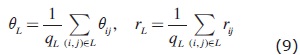
where θ_ij and r_ij are the intersection values from equations (4) and (5).

An additional advantage of this approach is that practical uncertainty estimates of the determined parameters can be calculated from the standard deviations of the intersection parameters. In what follows, the error margins indicated correspond to one standard deviation.

Figure 10 shows close-ups of the (automatic) cluster determinations for our example noisy alignments. The diamonds indicate the locations of the estimated parameters, where the short horizontal and vertical lines indicated the neighboring criteria (the same for both alignments) and crosses represent the intersections.

For Line 1, the estimated parameters are: θ_L1 = 131.830 ± 2.566º, and r_L1 0.221 ± 0.014 km, with qL1 = 33, which correspond to the line y = 0.297 ± 0.0009 + (0.895 ± 0.065)x. For Line 2, the estimated parameters are: θ_L2 = 68.649 ± 0.995º and r_L2 = 0.655 ± 0.009 km, with h_v = 18.382, q_L1 = 21, which correspond to the line y = 0.704 ± 0.015-(0.391 ± 0.020)x.

The resulting alignments are shown in Figure 11, together with (and for all practical purposes indistinguishable from) the true alignments.

A fortuitous alignment of the randomly positioned events is shown as a dashed line in figure 11.

 

Weighted Voting

The concept of weighted voting is an optional feature of the IHT and the CIHT, and can also be applied to the HT. It should be emphasized that weighted voting is not essential for intersective voting.

Usually the quality or reliability or representativity is not homogeneous for a given set of data, and this is always the case for geophysical data. For epicentral or hypocentral locations the goodness or reliability depends on many factors, such as the signal to noise ratio, the seismographic coverage, the character, impulsive or emergent, of seismic phase arrivals, etc.; because of this, locations of large earthquakes are usually more reliable than those of small earthquakes. Most location programs give estimates of inversion residuals and location quality or uncertainty. Also, large earthquakes that break large areas of a fault may be considered to be more representative of the fault.

Thus, weights can be assigned to data in order to ensure that results depend heavily on good data, while poor quality data can be made less important, or even irrelevant. So, let us suppose that each datum in physical space is assigned a weight, for the i'th point. Weights can take any values, but using weights in the [0, 1] range allows a straightforward interpretation of results. If no weighting is desired, then weights can be given all the same value (unity by preference).

For the data along the lines in the example set, weights have been assigned depending on the size of the mislocation errors, while non-aligned events have been assigned random weights. Data points physical space are plotted, from Figure 4 on, with symbol sizes proportional to their weights.

For the HT, instead of increasing by one the value in each accumulator cell the i'th curve crosses, the value is increased by the weight .

For both the IHT and the CIHT, the vote of each intersection, (θ_ij , r_ij) can be weighted as

so that intersections involving data with zero weight will have zero weight themselves, while intersections involving data having equal weights will have the same weight as each of the data.

For the IHT, Let w^c_mn be the sum of the weights of the intersections falling in the cell located in column m and row n, and let L be the set of indices of a group of (neighboring) cells containing all or most of the intersections from a given line. The total value assigned to the alignment is

and the alignment parameters can be estimated as

where θ^c_m and r^c_m are the θ and r values corresponding to the middle of the cells in column m and row n, respectively.

For the CIHT, if L is the set of indices of intersections belonging to a given cluster in Hough space, the alignment parameters can be estimated directly as:

the total weight associated with the cluster, and

where θ_ij and r_ij are the intersection values from equations (4) and (5).

For weights all equal to unity, equations (11) to (14) are equivalent to equations (6) to (9).

When using weights, both q_L and w_L can be used to have two slightly different characterizations or gradings of the estimated parameters, and the w_L / q_L ratio evaluates the relative quality of the data actually used for parameter identification.

Actually, the IHT and CIHT determinations shown above were done using weights, and the corresponding estimates are: w_l1 = 29.31 and w_L2 = 31.44 for the IHT, and w_L1 = 29.31 and w_L2 = 16.21 for the CIHT.

 

Conclusions

The Intersective Hough Transform (IHT), based on voting directly with the intersections of the cosenoids corresponding to each pair of points in observation space, yields a much clearer transform, where each non-zero value is significant. The IHT allows (much) smaller accumulation cells that can be grouped together to yield better estimates than those from the traditional Hough transform (HT). The Cluster Interceptive Hough Transform (CIHT) works without accumulator cells and allows estimating the uncertainty in the determination of each line; the CIHT can be completely automated.

Trials using synthetic data sets show that, for exact alignments, both IHT and CIHT give almost exact determinations, generally better than those from the traditional HT, even in the presence of noise consisting of large numbers of randomly located points. For inexact alignments the number of coinciding or clustering intercepts decreases according to the how much the locations depart from exact alignment; in some of these cases, and when random points are many, fortuitous alignments of random points may have total values larger than those of the desired alignments, but usually these are still recognizable. In all cases IHT and CIHT alignment identification performance is superior to that of the traditional HT.

 

Acknowledgments:

The author wishes to express his thanks to the reviewers and the editor.

 

References

Ballard D., 1981, Generalizing the Hough transform to detect arbitrary shapes. Pattern Recognition, 13 111-122.         [ Links ]

Duda R., Hart P., 1972, Use of the Hough transformation to detect lines and curves in pictures. Communications of the Association for Computing Machinery, 15 11-15.         [ Links ]

Fernandes L., Oliveira M., 2008, Real-time line detection through an improved Hough transform voting scheme. Pattern Recognition, 41 299-314.         [ Links ]

Furukawa Y., Shinagawa Y., 2003, Accurate and robust line segment extraction by analyzing distribution around peaks in Hough space. Computer Vision and Image Understanding, 92 1-25.         [ Links ]

Hart P., 2009, How the Hough transform was invented. IEEE Signal Processing Magazine 26 18-22.         [ Links ]

Hough P., 1959, Machine Analysis of Bubble Chamber Pictures. Proc. Int. Conf. High Energy Accelerators and Instrumentation, 1959.         [ Links ]

Illingworth J., Kitler J., 1988, A survey on the Hough transform. Computer Vision, Graphics, and Image Processing, 44 87-116.         [ Links ]

Kiryati N., Eldar Y., Bruckstein A., 1991, A probabilistic Hough transform. Pattern Recognition, 24 303-316.         [ Links ]

Li H., Lavin M., LeMaster R., 1986, Fast Hough transform: A hierarchical approach. Computer Vision, Graphics, and Image Processing, 36 139-161.         [ Links ]

O'Gorman F., Clowes M., 1976, Finding picture edges through collinearity of feature points. IEEE Transactions Computers, 25 449-45.         [ Links ]

Shapiro L., Stockman G., 2001, Computer Vision. Prentice-Hall, Inc.         [ Links ]

Wikipedia, http://en.wikipedia.org/wiki/Hough_transform. Accessed 20 November 2012.