


Servicios Personalizados
Revista
Articulo
 Inglés (pdf)
 Artículo en XML
 Referencias del artículo
 Enviar artículo por email
Indicadores
-
 Citado por SciELO
 -
 Accesos
Links relacionados
-
 Similares en
SciELO
Similares en
SciELO
Compartir

 Permalink
Geofísica internacional
versión On-line ISSN 2954-436Xversión impresa ISSN 0016-7169
Geofís. Intl vol.53 no.3 Ciudad de México jul./sep. 2014
Original paper
Edge enhancement in multispectral satellite images by means of vector operators
Jorge Lira* and Alejandro Rodríguez
Instituto de Geofísica, Universidad Nacional Autónoma de México Delegación Coyoacán, 04510 México D.F., México *Corresponding author: jlira@geociencias.unam.mx
Received: May 14, 2013.
Accepted: December 02, 2013.
Published on line: July 01, 2014.
Resumen
El realce de bordes es un elemento de análisis para entender la estructura espacial de imágenes de satélite. Se presentan dos métodos para extraer los bordes de imágenes multiespectrales de satélite. Una imagen multiespectral se modela como un campo vectorial de un número de dimensiones igual al número de bandas en la imagen. En este modelo, un pixel se define como un vector formado por un número d elementos igual al número de bandas. Se aplican dos operadores vectoriales a tal campo vectorial. En nuestro primer método, extendemos la definición de gradiente. En esta extensión, se obtiene el vector diferencia del pixel central de una ventana con los pixels vecinos. Se genera entonces una imagen multiespectral donde cada pixel representa el máximo cambio en la respuesta espectral en la imagen en cualquier dirección. A esta imagen se le denomina el gradiente multiespectral. El otro método considera la generalización del Laplaciano por medio de la transformada de Fourier h-dimensional. A esta imagen se le denomina el Laplaciano multiespectral. Los operadores vectoriales realizan una extracción simultánea del contenido de bordes en las bandas espectrales de la imagen multiespectral. Nuestros métodos son libres de parámetros. Nuestros métodos trabajan para una imagen multiespectral de cualquier número de bandas. Se discuten dos ejemplos que involucran imágenes multiespectrales de satélite a dos escalas. Comparamos nuestros resultados con procedimientos de realces de bordes ampliamente empleados. La evaluación de los resultados muestra un mejor comportamiento de los métodos propuestos comparados con los operadores de bordes ampliamente usados.
Palabras clave: detección de bordes, imagen multiespectral, realce de borde, operador vectorial.
Abstract
Edge enhancement is an element of analysis to derive the spatial structure of satellite images. Two methods to extract edges from multispectral satellite images are presented. A multispectral image is modeled as a vector field with a number of dimensions equal to the number of bands in the image. In this model, a pixel is defined as a vector formed by a number of elements equal to the number of bands. Two vector operators are applied to such vector field. In our first method, we extend the definition of the gradient. In this extension, the vector difference of the window central pixel with neighboring pixels is obtained. A multispectral image is then generated where each pixel represents the maximum change in spectral response in the image in any direction. This image is named a multispectral gradient. The other method, considers the generalization of the Laplacian by means of an η-dimensional Fourier transform. This image is named a multispectral Laplacian. The vector operators perform a simultaneous extraction of edge-content in the spectral bands of a multispectral image. Our methods are parameter-free. Our methods work for a multispectral image of any number of bands. Two examples are discussed that involve multispectral satellite images at two scales. We compare our results with widely used edge enhancement procedures. The evaluation of results shows better performance of proposed methods when compared to widely used edge operators.
Key words: edge detection, multispectral image, edge enhancement, vector operator.
Introduction
Edge detection has been undertaken for gray-level and color images using a number of methods and procedures. Most of the techniques published in the scientific literature in the last years deal with color images.
Well-established methods such as Kirsch, Sobel, Gradient and Laplacian operators have been widely used to extract edges in gray-level images (Pratt, 2001). Bowyer and co-workers (2001) provided a detailed account of a number of edge operators in gray images. The reviewed operators carry a set of parameters that needs to be defined in terms of heuristic criteria. Ground-truth images were used to derive a classification of edge operator performance (Bowyer et al., 2001). A deformable contour, defined by a wavelet snake, is designed to identify the boundary of pulmonary nodules in digital chest radiographs (Yoshida, 2003). In this work (Yoshida 2003), a multi-scale edge representation is obtained by means of the wavelet transform; this produces, however, fragmented edge segments. Therefore, a wavelet snake was used to produce a smooth and closed contour of a pulmonary nodule.
Other methods to detect edges in gray-level images use fuzzy logic. Segmentation of a fuzzy image into regions of similar image properties was achieved by means of a fuzzy procedure (Bigand et al., 2001). This method works with fuzzy-like and noisy images. Zero crossings that correspond to gradient maxima were obtained by means of the cosine transform in noisy images (Sundaram, 2003). This scheme favors the detection of weak edges in background noise and suppresses false edges.
The modeling of natural RGB images as vector fields has been exploited to detect edges in color images (Koschan and Abidi, 2005; Evans and Liu, 2006). In their studies, the authors (Koschan and Abidi, 2005) provide an overview of color edge detection techniques, and, in particular, generalizations of Canny and Cumani operators to color spaces were discussed with examples. Evans and Liu (2006) provide a review of color edge detectors.
A parameter-free approach could be obtained when an automatic determination threshold was calculated using a model-based design (Fan et al., 2001). With this approach, a color-image edge operator is derived. Cellular neural networks applied to color images resulted in a model to detect edges (Li et al., 2008). This model was successfully applied to RGB images with color test patterns. In addition to these results, the authors provided a detailed revision of color edge detection techniques.
Recent advances in edge enhancement for color images show clear advantages over methods for mono-spectral images (Xu et al., 2010; Chen and Chen, 2010; Nezhadarya and Kreidieh, 2011; Gao et al., 2011; Chu et al., 2013). Color images are increasingly used in many applications such as surveillance, computer vision and robotics. Multispectral satellite images are available at several scales. For these two groups of images, edge enhancement is an element of structural analysis.
A general method is needed that works for any number of bands, with no parameters and a reasonable computing time. To fulfill such goal, we model a multispectral satellite image by means of a vector field. The dimension of this field equals the number of bands of the image. Upon this field, we may apply vector operators. We compare our results with those obtained from conventional edge operators (Pratt, 2001; Bowyer et al., 2001). We carry out a detailed evaluation of our results. Such evaluation includes qualitative and quantitative analysis. Our evaluation shows a clear improvement with respect to conventional edge operators.
Study area and data
Two multispectral satellite images were used to test the goodness of our method at different scales. Both images cover a portion of Mexico City where the runaways of an airport are clearly visible. One of the images is formed by the visible and near infrared (VNIR) bands of the Advanced Spaceborne Thermal Emission and Reflection Radiometer sensor (ASTER) on board Terra satellite (Figure 1). The four bands of the IKONOS sensor (Figure 2) form the other image. Table 1 provides basic parameters of these images.

The high density of streets, avenues and buildings of the city results in a large number of edges per unit area. Such edges are of varying shape and size. Therefore, the multiple edges formed by streets, avenues, causeways and building blocks are a good test for our method.
These images are not precisely orthorectified since no implications on our method arise. However, rectification with first-order polynomial equation was applied in order to relate pixel coordinates with geographic coordinates.
Methods
In a multispectral image, the information-content of edges varies through the bands. In order to extract the information of edges from the multispectral image, we require a transformation applicable to the image as a whole.
In addition to the original bands, principal components analysis was performed on the two images. The first principal component of both images is used to apply widely used edge operators (Pratt, 2001; Bowyer et al., 2001). These operators are used for the sake of comparison with the methods developed in our work. The first principal component accumulates most of the variance of the images: 78.50% for the ASTER image, and 83.09% for the IKONOS image. Therefore, we applied widely used edge operators to the first principal component.
Vector field of a multispectral image
The modeling of an h-dimensional multispectral image as a vector field will be addressed in section 3.1 (Lira and Rodríguez, 2006). This field holds the same dimension as the original multispectral image. The field is composed by the set of pixels considered as h-dimensional vectors.
In Section 3.2, we determined maximum difference vectors in a moving window that systematically scan the entire image. This maximum difference produces an h-dimensional image where edges are enhanced.
In Section 3.3, we derived an h-dimensional Laplacian using Fourier transform. To do so, we first consider the Fourier transform of second partial derivates of an image (Bracewell, 2003). With this result, we produced the Laplacian of an image. Finally, we generalized the Laplacian for multispectral images composed of h-bands. A flow chart resumes our methods, from the modeling of a multispectral image as a vector field, to the enhancement of edges through the bands of the image (Figure 3)

Let L ≡ {1, . . . M} • {1, . . . N} be a rectangular discrete lattice. This lattice is virtually overlaid on the scene. On each node of L, a resolution cell named the instantaneous field of view (IFOV) is located. For each IFOV, an h-dimensional vector {b1,b2, . . . bη} is derived by means of a multispectral sensor set. The vector {b1,b2, . . . bη} represents the average spectral properties of an IFOV of the scene. This vector is named a picture element (pixel) of a multi-spectral image. In other words, the IFOV is a physical area in the scene, while the pixel is the digital number (DN) in the image. Let the multi-spectral image g = {gi} be formed by the group of pixels according to the following set gi = {bj(k,l)}i, ∀ i. Where i ∈ ℕ is the set {1,2, . . . η} representing the collection of bands of the multispectral image.
On the other hand, let Xi be the set

Where m =8 in most cases. The cartesian product Xη = X1 × X2 × . . . Xη defines the set of the ordered η-tuple (x1,x2, . . . xη). We equate xi = bi, therefore (b1,b2, . . . bη) is an η-tuple in this cartesian coordinate system. To every h-tuple (b1,b2, . . . bh), a vector u is associated: u(x1,x2, . . . xη) ⇐ (b1,b2, . . . bη).
The set of vectors {u(x1,x2, . . . xη)} is the result of the mapping of the multispectral image onto a vector field. We note that not every h-tuple (x1,x2, . . . xη), has a vector associated to the vector field, and an n-tuple (x1,x2, . . . xη) may have more than one vector associated to the vector field. Hence, the vector field associated with the multispectral image is the set of vectors U = {u(x1,x2, . . . xη)}.
Multispectral gradient
Once the multispectral image is modeled as a vector field, we may proceed to define a multispectral edge. Let vc be a moving window that systematically scans, pixel by pixel, the whole image. The window vc is of size 3×3 pixels. Let D(g) be the domain of the image, thus the condition that vc ⊂ D(g) determines that the border pixels of the image cannot be processed.
Let the vector pc be the central pixel of such window and let p1, p2, . . . p8 be the neighboring pixels of pc. The set of pixels {pi}, i = 1, 2, . . . 8 is the 8-connected neighbor set of pc. We obtain the vector difference of the central pixel with all neighboring pixels of the window

The vector of the window that makes the largest difference is written in an output multispectral image named f

Equation (3) means that central pixel pc, in moving window, is replaced by neighboring pixel pi with the largest Euclidiean distance to the central pixel.
The vector difference is calculated employing the Euclidian distance

The image f contains the edge information across the bands of the original image g. Image f is dubbed the multispectral gradient (Figure 3).
Average of bands of output edge image f is calculated in order to concentrate the information on a single image. Principal components analysis may be applied as well to output image f to concentrate in the first component the edge content of the multispectral-edge image. We use the average of the output image bands.
Derivation of η-dimensional Laplacian
A Laplacian is widely used as an edge operator (Pratt, 2001). Nevertheless, actual Laplacian is applied to each separate band of a multispectral image. A multispectral Laplacian is needed to extract edge content from the ensemble of the bands as a whole.
We begin with the consideration of the Laplacian in continuous space, and then we write the result in discrete space. Let g(x,y) ∈ℝ2 be a function that describes a single band image where (x,y) are the coordinates of a pixel in this image. We initiate this step with the use of the equations

A detailed explanation on the derivation of equations (5) and (6) is provided in Lira (2010). In equations (5) and (6), ℱ stands for Fourier transform, G(ωx,ωy) is the Fourier transform of the image g(x,y) and j is the complex number √-1. In equations (5) and (6), (x,y) are spatial coordinates in image domain, whereas (wx, wy) are spatial frequencies in Fourier domain.
From equations (5) and (6) we have the Fourier transform of the Laplacian

Equation (7) is dubbed the scalar Laplacian.
On the grounds of results given by equation (7), we may generalize the Fourier transform of the Laplacian to n-dimensions. Let f(r) ∈ℝη, be a vector valued function that describes a multispectral image formed by n-bands. The vector f(r) = {f1(x,y), f2(x,y), . . . fη(x,y)} represents the values of a pixel through the bands, i.e., the image value at a pixel location r = (x,y) ∈ ℝη. The function f(r) is a vector field that describes the multispectral image according to lineaments described in section 3.1 (Lira and Rodriguez, 2006). The Fourier transform of f(r) is then (Bracewell, 2003; Ebling and Scheuermann, 2005)

The Fourier transform of the vector field f(r) produces a vector valued ℱ function in Fourier space, namely, F(ω) = [f(r)]. The vector F(ω) = {F1(ω1, ω2), F2(ω1, ω2), . . . Fη(ω1, ω2)}, represents the spatial frequency content of the image at the location ω = (ω1,ω2). In ℝη, the coordinates in Fourier domain (w1, w2), and spatial domain (x, y), cover the same range, 1 ≤ (x, w1) ≤ M and 1 ≤ (y, ω2) ≤ N, but their meaning is different: (x, y) represents spatial coordinates, while (ω1, ω2) represents spatial frequencies.
In discrete space ℤη, the coordinates in Fourier domain k = (k1, k2), and spatial domain q = (m, n), cover the same range, 1 ≤ (m, k1) ≤ M and 1 ≤ (n, k2) ≤ N. If f(q) ∈ ℤη, where (m, n; k1, k2) ∈ ℤη, then the discrete version of equation (8) is
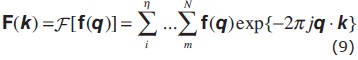
Where f(q) = {f1(m, n), f2(m, n), . . . fh(m, n)} and F(k) = {F1(k1, k2), F2(k1, k2), . . . Fη(k1, k2)}. The Laplacian in ℤη of the vector field f(q) is therefore

Where F(k) = [f(q)]. This equation can be applied to a multispectral image to derive edge content through the bands. Note that equation (7) is a particular case of equation (10). Equation (10) is dubbed the multispectral Laplacian.
To calculate this multispectral Laplacian, we first obtain the Fourier transform of the vector field associated to the image to produce F(k). In Fourier space, we multiply the result by – (2π)2│k│2 and apply the inverse Fourier transform to obtain the multispectral Laplacian (Figure 3).
Evaluation of edges
The criteria to evaluate the edge enhancement resulting from our methods and from widely known edge operators are divided in qualitative and quantitative. The edges produced by the urban network of streets, avenues, buildings, idle lots and parks occur at random directions in the images. Due to this randomness, a profile of pixel values along any direction is representative of the edge content of the images. We considered pixel values profiles along several directions. We analyzed such profiles for widely known edge operators and for outputs of our methods. We present the plots of two profiles for each sensor, and we include two graphs that condense the behavior of ten profiles for each sensor: ASTER and IKONOS. In total, we analyzed twenty profiles. From these plots, we derive a qualitative and quantitative evaluation as described below. Black dots in figures 5, 6, 7, and 8 indicate the lines where the plots were extracted. Figures 11, 12, 13, and 14 indicate the line, column and angle of the location of profiles.
Qualitative evaluation
We display in a high-resolution monitor the edge enhanced images. We display as well the first principal component of both images. A detailed visual inspection is carried out. On the grounds of previously published work on qualitative image evaluation (Escalante-Ramirez and Lira, 1996), each edge-enhanced image was rated according to the following qualitative criteria: general quality, sharpness, contrast, and noisiness. In addition, we evaluated the number of gray levels and definition of edges. Since the first principal component of the images accumulates most of the variance, we compare the edge enhancement with this component. The aim of this comparison is to evaluate, according to the above criteria, the degree of edge enhancement with respect to the original edge information content of the images.
Quantitative evaluation
We use several indicators to perform a quantitative evaluation (Figure 4): Slope – the more steepness the better the definition of the slope of an edge. Widening – a width as close as possible to the original edge the better. Spatial location – the closest of the enhanced edge to the original location the better. Contrast – the highest the contrast the better.
A computer code was developed for quantitative evaluation. An image is displayed in a high resolution monitor. With the help of a cursor, a line of the image is selected. The profile of pixel values is shown in a plot. A profile is selected that contains one of the edge models given in figure 4. A spline is obtained for the selected edge-model. From such spline, the parameters indicated in the models of figure 4 are calculated. There are many types of edges in the images. To obtain a coherent quantitative evaluation of edges, we considered three types that occur frequently in the images. Figure 4 shows a schematic diagram of such types where the above indicators are depicted. We performed such measurement for an ensemble of edges. Figure 4(c) shows a profile that occurs only in Laplacian and Kirsch operators. The computation of indicators is as follows.
Slope – we measure the slope as the angle of the borders of an edge with respect to the vertical direction. Widening – we measure the maximum width of an edge in pixels. Spatial location – we identify the spatial coordinate of the center of an edge. Contrast – we measure the contrast as the difference between the maximum value and the minimum value of an edge.
In order to complement our evaluation of edge enhancement we developed a computer code for the Canny and Cumani operators (Koschan and Abidi, 2005; Evans and Liu, 2006). The computer code was designed following the method explained in the article by Koschan and Abidi (2005). Two RGB false color composites were produced using the first three bands of ASTER and IKONOS images. Upon these images, the Canny and Cumani operators were applied. Such operators consist of a two-step procedure. The first step is the enhancement of the edges; the second step is the detection of the edges by means of a threshold operation. We present results only for the enhancement of the edges. Both operators, Canny and Cumani, carry a number of parameters that require a determination by heuristic procedures. There are no analytical methods to estimate such parameters in an optimal design. Instead, our methods are parameter-free.
Results and discussion
Results
The necessary algorithms to apply the methods described in previous section were developed using Delphi language running under Windows 7 in a PC. Several edge products are presented in our work. They are organized in two groups: (a) edges from widely used edge operators, (b) edges derived from the methods developed in our work. These groups are analyzed. In order to facilitate the comparison of these results, four mosaics of selected regions of the images were prepared. These mosaics include the multispectral edges derived from our method and results from the above mentioned edge operators. Boxes on figures 1 and 2 show the areas from which these mosaics were extracted. The mosaic prepared from boxes on the left of figures 1 and 2 are dubbed mosaic A, and those on the right are dubbed mosaic B.
A set of profiles are produced to evaluate the performance of edge enhancement of the methods compared in this research. Profiles are compared. A profile from the first principal component of the original image is compared against the profiles of all edge enhancement methods considered in our work.
The mosaics are used to perform the qualitative evaluation as discussed in previous section. The profiles are used to develop the quantitative evaluation as discussed in previous section. The above-mentioned groups show the following results.
1) Edges from vector differences in a moving window (multispectral gradient).
As explained in Section 3.1, a multispectral edge image is obtained. This multispectral image carries the same number of bands as the input image. The average of the bands of such multispectral edge image was used for quantitative evaluation. Figures 5 and 6 shows the enhancement of edges of the ASTER image resulting from such procedure. Figures 7 and 8 depict the enhancement of edges of the IKONOS image. For visual purposes, a linear saturation enhancement was applied to figures 5 - 8. The quantitative evaluation was performed upon original results.
2) Edges from the multispectral Laplacian (Section 3.2).
The multispectral Laplacian derived from equation (10) was applied to both images, ASTER (figures 5 and 6) and IKONOS (figures 7 and 8).
3) Edges from the first principal component of images.
The following edge operators were applied to the first principal component of ASTER and IKONOS images: Sobel, Frei-Chen, Kirsch, scalar Laplacian, Prewitt and Roberts. Results are shown in figures 5 and 6 for ASTER image, and figures 7 and 8 for IKONOS image.
4) Edges from color operators
Two mosaics were prepared to show the results of Canny and Cumani operators (Figure 9). We applied a histogram saturation transformation to the images of the mosaics for visual appreciation purposes. An inspection of results shows an enhancement similar to the Sobel operator (Figure 6). There are two limitations to the Canny and Cumani operators. The first one is that they carry a number of parameters that need to be defined by experimental procedure. The second one is that they work for RGB color images only; no generalization exists for an arbitrary number of bands of a multispectral image.
The profiles for all edge enhancement methods are shown in figures 11 and 12 for ASTER mosaics and figures 13 and 14 for IKONOS mosaics.
In order to complement the procedure of profile extraction (Figures 11 - 14), a mosaic of strip-images was prepared (Figure 10). The strip consist of a sub-image of 21 pixels long by 11 pixels wide. The dots indicate the line of pixels related to the profile. The mosaic is formed by 6 strips, one for each image of figure 6. We present one mosaic of strips.
5) The indicators (Figure 4) described in quantitative evaluation were measured for twenty profiles: ten for ASTER image and ten for IKONOS image. The measurement was carried out for the whole ensemble of edge operators considered in our research. Such measurement includes the first principal component of ASTER and IKONOS images. The value of the indicators was compared with the value of the original profile extracted from the first principal component. This comparison was calculated in relative error percentage and condenses in a single graph. The relative error percentage is the difference of an indicator from an edge enhanced image (Ie) minus the indicator from the first principal component (Icp) normalized by (Icp). Figure 15 shows the graph that summarizes the quantitative evaluation of the profiles. For ASTER image, figure 15(a) depicts the relative error percentage with respect to the original profile in first principal component. Figure 15(b) show results for IKONOS image. Angles q1 and q2 are not included in figure 15 for multispectral Laplacian and for Kirsch operators since, as explained above, the profile of figure 4(c) does not occur in the original image. Such operators introduce an inversion of contrast described in figure 4(c). None the less, the profile-type of figure 4(c) was compared among multispectral Laplacian and Kirsh operators. The contrast for all operators is presented in figure 16 for both sensors.
Discussion
Our discussion is divided in qualitative and quantitative evaluation as described in Section 3.4. The next two sections provide detailed description of such evaluation.
Qualitative discussion
A visual inspection of results, using the qualitative criteria described in Section 3.3, produces higher rating for our methods in comparison with any other edge-enhancement method considered in our research. For such inspection, we employed figures 5 to 8. In particular, and on the grounds of such rating, we may list the following evaluation
(a) Edges from Sobel, Frei-Chen, Prewitt and Roberts operators are widened for both images. The images from these operators appear unsharpened. The contrast is high and has a noisy appearance. Thin lines, points and linear objects are blurred or obliterated.
(b) Edges from the Kirsch operator show a relief-like appearance of urban buildings structure. The relief-like appearance is derived from the second derivative involved in the definition of this operator. Results look somewhat unsharpened and contrast is relatively small. There is no noisy appearance. Thin edges, points and linear objects are blurred.
(c) Edges from the scalar Laplacian operator are less widened than other operators. Results are sharp, thin edges, points and linear objects are preserved. However the contrast is low. No-noisy appearance is observed.
(d) The average of the bands of the image resulting from the multispectral gradient show sharp edges with good contrast. The contrast is higher than the scalar gradient, details such as thin lines and points are preserved. No noisy appearance is observed.
(e) The edge image resulting from the multispectral Laplacian show a relief-like appearance with better definition and similar than the Kirsch operator. The relief appearance of the multispectral Laplacian is sharpening with better preservation of fine details than the scalar Laplacian. The contrast is high and edges are sharp. No noise is observed.
(f) The sharpness of edges, the contrast, the noisiness appearance, and general quality of multispectral gradient and multispectral Laplacian are better than the edge operators compared in our work (Figure 15).
Quantitative discussion
As shown in figures 5 - 8, the dots on the border of the mosaics indicate the lines were pixel values profiles are extracted. These lines were selected to include sharp edges such as the lines of the landing fields of the airport and abrupt change of pixel values due to constructions or particular features with high contrast. The profiles extracted from the first principal component are compared to the profiles extracted form edge enhancement images. Many profiles were inspected at random. A selection of profiles was performed when they contained at least one of the edge-models of figure 4. We measured the above-described indicators (Figure 4) for twenty selected edge profiles: those with the best definition. From such measurements, we derived a list of conclusions.
Profiles of selected lines of the ASTER and IKONOS image-mosaics show the following:
(1) Sobel, Frei-Chen and Roberts operators wide and smooth the profiles of the original edges of the images.
(2) Kirsch and Prewitt operators wide and smooth the profiles but in a less degree than Sobel, Frei-Chen and Roberts operators.
(3) The relief-like appearance of the Kirsch images is due to the contrast inversion of some edges of the original profile.
(4) The scalar Laplacian operator does not wide nor smoothes the edges but reduces the contrast of the edges.
(5) The multispectral gradient and the multispectral Laplacian do not wide nor smooth the edges, and in addition to this, increase the contrast of the edges.
(6) The multispectral gradient and the multispectral Laplacian show good contrast of the enhanced edges.
(7) The spatial location error is highest for Roberts operator. The least error is for the scalar Laplacian.
(8) The steepness of the enhanced edges is less than the original edges for those operators that smooth and wide the edges.
(9) Overall, the multispectral gradient and the multispectral Laplacian show good conditions of contrast, steepness, spatial location and definition of edges with respect to the other operators.
Possible applications for multispectral edge enhancement are: identification of linear feature for geologic environments, identification of ancient highways in archeological studies, delineation of coastlines, studies of urban structures, delineation of water bodies and studies of coastal current patterns.
Conclusions
Two methods to extract edges from multispectral images are designed and discussed in this research. Such methods require the modeling of the original multispectral image as a vector field. Upon this vector field, we applied two vector operators to extract the edge content originally distributed through the bands of the images. These methods are parameter-free. A qualitative and quantitative evaluation show that our methods perform better than widely used edge enhancement procedures. The basic reason for this is that our methods extract the edge-content distributed through the original bands of a multispectral image. Our methods are not computing demanding, we use a fast Fourier transform to calculate the multispectral Laplacian. The calculation of the multispectral gradient is fast since it involves vector differences in a moving window. On a PC under Windows 7, the computing time for a 2000 ´ 2000 pixels multispectral image with 6 bands does not exceed three minutes. Our methods work for multispectral images with any number of bands, the limit is set by the available memory. A test on hyperspectral images is not yet performed.
References
Bigand A., Bouwmans T., Dubus J.P., 2001, Extraction of line segments from fuzzy images, Pattern Recognition Letters, 22, 13, 1405 – 1418. [ Links ]
Bowyer K., Kranenburg C., Doughert S., 2001, Edge detector evaluation using empirical ROC curves, Computer Vision and Image Understanding, 84, 1, 77 – 103. [ Links ]
Bracewell R.N., 2003, Fourier Analysis and Imaging, Kluwer Academic, New York. [ Links ]
Chen X., Chen H., 2010, A novel color edge detection algorithm in RGB color space, IEEE 10th International Conference on Signal Processing, Beijin, China, pp. 793 - 796. [ Links ]
Chu J., Miao J., Zhang G., Wang L., 2013, Edge and corner detection by color invariants, Optics and Laser Technology, 45, 756 - 762. [ Links ]
Ebling J., Scheuermann J., 2005, Clifford Fourier transform on vector fields, IEEE Transactions on Visualization and Computer Graphics, 11, 469 – 479. [ Links ]
Escalante-Ramírez B., Lira J., 1996, Perfor-mance-oriented analysis and evaluation of modern adaptive speckle reduction techniques in SAR images, Proceedings, SPIE's Visual Information Processing V, Orlando, Florida, 2753, pp. 18-27. [ Links ]
Evans A.N., Liu X.U., 2006, A morphological gradient approach to color edge detection, IEEE Transactions on Image Processing, 15, 1454 - 1463. [ Links ]
Fan J.P., Aref W.G., Hacid H.S., EL Maguimid A.K., 2001, An improved automatic isotropic color edge detection techniques, Pattern Recognition Letters, 22, 13, 1419 – 1429. [ Links ]
Gao C.B., Zhou J.L., Hu J.R., Lang F.N., 2011, Edge detection of colour image based on quaternion fractional differential, IET Image Processing, 5, 261 - 272. [ Links ]
Koschan A., Abidi M., 2005, Detection and classification of edges in color images, IEEE Signal Processing, 22, 1, 64 – 73. [ Links ]
Li G.D., Min L.Q., Zang H.Y., 2008, Color edge detections based on Cellular Neural Network, International Journal of Bifurcation and Chaos, 18, 4, 1231 – 1242. [ Links ]
Lira J., Rodríguez A., 2006, A Divergence Operator to Quantify Texture From Multi-spectral Satellite Images, International Journal of Remote Sensing, 27, 2683 – 2702. [ Links ]
Lira J., 2010, Tratamiento Digital de Imágenes Multiespectrales, www.lulu.com [ Links ]
Nezhadarya E., Kreidieh R., 2011, A new scheme for robust gradient vector estimation on color image, IEEE Transactions on Image Processing, 20, 2211 - 2220. [ Links ]
Pratt W.K., 2001, Digital Image Processing, Wiley Interscience, New York. [ Links ]
Sundaram R., 2003, Analysis and implementation of an efficient edge detection algorithm, Optical Engineering, 42, 642 – 650. [ Links ]
Xu J., Ye L., Luo W., 2010, Color edge detection using multiscale quaternion convolution, International Journal of Imaging Systems and Technology, 20, 354 - 358. [ Links ]
Yoshida H., 2003, Multiscale edge-guided wavelet snake model for delineation of pulmonary nodules in chest radiographs, Journal of Electronic Imaging, 12, 1, 69 – 80. [ Links ]

