Original paper

 

Neural estimation of strong ground motion duration

 

Leonardo Alcántara Nolasco*, Silvia García, Efraín Ovando-Shelley and Marco Antonio Macías Castillo

 

Instituto de Ingeniería, Universidad Nacional Autónoma de México, Delegación Coyoacán, 04510, México D.F., México *Corresponding author: leonardo@pumas.ii.unam.mx

 

Received: November 09, 2012.
Accepted: November 19, 2013.
Published on line: July 01, 2014.

 

Resumen

Este artículo presenta y discute el uso de las redes neuronales para determinar la duración de los movimientos fuertes del terreno. Para tal efecto se desarrolló un modelo neuronal, utilizando datos acelerométricos registrados en las ciudades mexicanas de Puebla y Oaxaca, que predice dicha duración en términos de la magnitud, distancia epicentral, profundidad focal, caracterización del suelo y el azimut. Por lo que, el modelo considera los efectos tanto de la zona sismogénica como del tipo de suelo en la duración del movimiento. El esquema final permite una estimación directa de la duración a partir de variables de fácil obtención y no se basa en hipótesis restrictivas. Los resultados presentados en este artículo indican que la alternativa del cómputo aproximado, particularmente las redes neuronales, es una poderosa aproximación que se basa en los registros sísmicos para explorar y cuantificar los efectos de las condiciones sísmicas y de sitio en la duración del movimiento. Un aspecto esencial y significante de este nuevo modelo es que a pesar de ser extremadamente simple ofrece estimaciones de duración con notable eficiencia. Adicional e importante son los beneficios que arroja esta simplicidad sobre la separación natural de los efectos de la fuente, patrón o directividad y de sitio además de la eficiencia computacional.

Palabras clave: duración del movimiento de terreno, parámetros de movimientos de terreno, duración significativa, intensidad de Árias, redes neuronales, cómputo aproximado.

 

Abstract

This paper presents and discusses the use of neural networks to determine strong ground motion duration. Accelerometric data recorded in the Mexican cities of Puebla and Oaxaca are used to develop a neural model that predicts this duration in terms of the magnitude, epicenter distance, focal depth, soil characterization and azimuth. According to the above the neural model considers the effect of the seismogenic zone and the contribution of soil type to the duration of strong ground motion. The final scheme permits a direct estimation of the duration since it requires easy-to-obtain variables and does not have restrictive hypothesis. The results presented in this paper indicate that the soft computing alternative, via the neural model, is a reliable recording-based approach to explore and to quantify the effect of seismic and site conditions on duration estimation. An essential and significant aspect of this new model is that, while being extremely simple, it also provides estimates of strong ground motions duration with remarkable accuracy. Additional but important side benefits arising from the model's simplicity are the natural separation of source, path, and site effects and the accompanying computational efficiency.

Key words: strong ground motion duration, ground motion parameters, significant duration, Árias Intensity, neural networks, soft computing.

 

Introduction

The principal objective of engineering seis-mology is to supply quantitative estimations of expected ground-motions for earthquake-resistant design, evaluation of seismic hazards, and seismic risk assessment through the proper characterization of complex time series (accelerograms). Since the first strong-motion accelerograms were recorded a large number of parameters have been defined to characterize movements. The usefulness of strong-motion parameters is dependent primarily upon their intended use. The parameters that can be employed in earthquake-resistant design are few and are directly related to the methods of structural analysis used in current practice. Once a parameter has been selected to characterize the ground motion, it is necessary to develop relationships between this parameter and important seismic features as earthquake source, travel path, and site conditions.

The essence of such predictive relationships for the duration of strong motions depends very heavily on the way duration is defined. In fact many strong-motion duration definitions have been presented; however, all of them attempt to isolate a certain portion of the time series where strongest motion occurs. In general terms, it has been accepted that all of these definitions can be grouped into one of four generic categories (Bommer and Martínez-Pereira, 1996): i) the bracketed duration, the interval between the first and last excursion of particular threshold amplitude, ii) the uniform duration, the sum of all of the time intervals during which the amplitude of the record is above the threshold, iii) the significant duration, which is determined from the Husid plot (Husid, 1969) based on the interval during which a certain portion of the total Árias intensity is accumulated and iv) the structural response duration, determined by applying one of the above three categories to the response of a specific single-degree-of-freedom oscillator.

In this investigation, and considering the definition of significant duration, the connection between data and knowledge is found using a soft computing SC tool: the neural networks NNs. This alternative improves the theory and understanding of the driven parameters (of all kinds including indeterminate ones, possibly expressed in words) of ground-motion duration behavior. SC, NNs particularly, utilize a discovery approach to examine the multidimensional data relationships simultaneously and to identify those that are unique or frequently represented, permitting the acquisition of structured knowledge.

A neuronal empirical model for strong motion duration is proposed here, derived from seismic information registered in Puebla and Oaxaca, México. This model predicts the strong ground motion duration as a function of earthquake magnitude, epicentral distance, focal depth, azimuth (established from epicenters to stations) and soil characterization. The final scheme permits a direct estimation of the duration since it requires easy-to-obtain variables and does not have restrictive hypothesis

 

Soft Computing

The term Soft Computing SC represents the combination of emerging problem-solving technologies such as Fuzzy Logic FL, Probabilistic Reasoning PR, Neural Networks NN, and Genetic Algorithms GAs. Each of these provides complementary reasoning and searching methods to solve complex, real-world problems. In ideal problem formulations, the systems to be modeled or controlled are described by complete and precise information. In these cases, formal reasoning systems, such as theorem proofs, can be used to attach binary true or false values to statements describing the state or behavior of the physical system.

Soft Computing technologies are flexible computing tools to perform these approximate reasoning and search tasks handling imperfect information. According to Zadeh (Fuzzy Logic pioner): ''...in contrast to traditional, hard computing, soft computing is tolerant of imprecision, uncertainty, and partial truth.'' The only obvious common point between SC tools (Fuzzy Logic FL, Neural Networks NNs and Genetic Algorithms GAs) is that they have been inspired by the living: the imprecision of human language and its efficiency in conveying and transmitting information for FL, the architecture of the brain for NNs, and the reproduction of living beings for GAs.

Neural Networks

This section will briefly explain the theory of neural networks NN. For a more in depth explanation of these concepts consult Hassoun, (1995); Hertz et al., (1991) and Tettamanzi and Tomassini, (2001).

In the brain, a NN is a network consisting of connected neurons. The nucleus is the center of the neuron and it is connected to other nuclei through the dendrites and the axon. This connection is called a synaptic connection. The neuron can fire electric pulses through its synaptic connections, which are received by the dendrites of other neurons. Figure 1 shows how a simplified neuron looks like. When a neuron receives enough electric pulses through its dendrites, it activates and fires a pulse through its axon, which is then received by other neurons. In this way information can propagate through the NN. The synaptic connections change throughout the lifetime of a neuron and the amount of incoming pulses needed to activate a neuron (the threshold) also change. This process allows the NN to learn (Tettamanzi and Tomassini, 2001).

Mimicking the biological process the artificial NN are not "intelligent" but they are capable for recognizing patterns and finding the rules behind complex data-problems. A single artificial neuron can be implemented in many different ways. The general mathematic definition is given by equation 1.

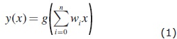
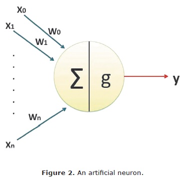
where x is a neuron with n input dendrites (x₀,..., x_n) and one output axon y(x) and (w₀,...,w_n) are weights determining how much the inputs should be weighted; g is an activation function that weights how powerful the output (if any) should be from the neuron, based on the sum of the input. If the artificial neuron mimics a real neuron, the activation function g should be a simple threshold function returning 0 or 1. This is not the way artificial neurons are usually implemented; it is better to have a smooth (preferably differentiable) activation function (Bishop, 1996). The output from the activation function varies between 0 and 1, or between -1 and 1, depending on which activation function is used. The inputs and the weights are not restricted in the same way and can in principle be between -∞ and +∞, but they are very often small values centered on zero (Broomhead and Lowe, 1988). Figure 2 provides a schematic view of an artificial neuron.

As mentioned earlier there are many different activation functions, some of the most commonly used are threshold (Eq. 2), sigmoid (Eq.3) and hyperbolic tangent (Eq.4).

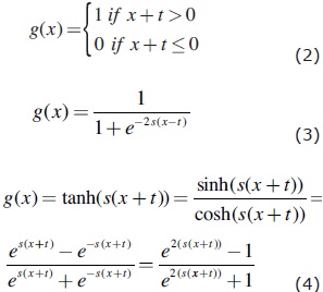
where t is the value that pushes the center of the activation function away from zero and s is a steepness parameter. Sigmoid and hyperbolic tangent are both smooth differentiable functions, with very similar graphs. Note that the output range of the hyperbolic tangent goes from -1 to 1 and sigmoid has outputs that range from 0 to 1. A graph of a sigmoid function is given in Figure 3 to illustrate how the activation function looks like. The t parameter in an artificial neuron can be seen as the amount of incoming pulses needed to activate a real neuron. A NN learns because this parameter and the weights are adjusted.

NN architecture

The NN used in this investigation is a multilayer feedforward neural network MFNN, which is the most common NN. In a MFNN, the neurons are ordered in layers, starting with an input layer and ending with an output layer. There are a number of hidden layers between these two layers. Connections in these networks only go forward from one layer to the next (Hassoun, 1995). They have two different phases: a trai-ning phase (sometimes also referred to as the learning phase) and an execution phase. In the training phase the NN is trained to return a specific output given particular inputs, this is done by continuous training on a set of data or examples. In the execution phase the NN returns outputs on the basis of inputs. In the NN execution an input is presented to the input layer, the input is propagated through all the layers (using equation 1) until it reaches the output layer, where the output is returned. Figure 4 shows a MFNN where all the neurons in each layer are connected to all the neurons in the next layer, what is called a fully connected network.

Two different kinds of parameters can be adjusted during the training, the weights and the t value in the activation functions. This is impractical and it would be easier if only one of the parameters were to be adjusted. To cope with this problem a bias neuron is introduced. The bias neuron lies in one layer, connected to all the neurons in the next layer, but none in the previous layer and it always emits 1. A modified equation for the neuron, where the weight for the bias neuron is represented as w_n+1, is shown in equation 5.

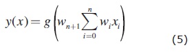
Adding the bias neuron allows the removal of the t value from the activation function, leaving the weights to be adjusted, when the NN is being trained. A modified version of the sigmoid function is shown in equation 6.

The t value cannot be removed without adding a bias neuron, since this would result in a zero output from the sum function if all inputs where zero, regardless of the values of the weights

Training a NN

When training a NN with a set of input and output data, we wish to adjust the weights in the NN to make the NN gives outputs very close to those presented in the training data. The training process can be seen as an optimization problem, where the mean square error between neural and desired outputs must be minimized. This problem can be solved in many different ways, ranging from standard optimization heuristics, like simulated annealing, to more special optimization techniques like genetic algorithms or specialized gradient descent algorithms like backpropagation BP.

 

The backpropagation algorithm

The BP algorithm works in much the same way as the name suggests: after propagating an input through the network, the error is calculated and the error is propagated back through the network while the weights are adjusted in order to make the error smaller. Although we want to minimize the mean square error for all the training data, the most efficient way of doing this with the BP algorithm, is to train on data sequentially one input at a time, instead of training the combined data.

BP application steps. First the input is propagated through the NN to the output. Then the error ek on a single output neuron k can be calculated as:

where y_k is the calculated output and d_k is the desired output of neuron k. This error value is used to calculate a δ_k value, which is again used for adjusting the weights. The δ_k value is calculated by:

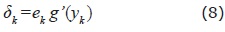
where g' is the derived activation function. When the δ_k value is calculated, the δ_j values can be calculated for preceding layers. The δ_j values of the previous layer are calculated from the δ_k values of this layer by the following equation:

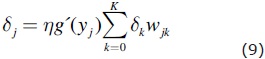
where K is the number of neurons in this layer and η is the learning rate parameter, which determines how much the weight should be adjusted. The more advanced gradient descent algorithms does not use a learning rate, but a set of more advanced parameters that makes a more qualified guess to how much the weight should be adjusted. Using these δ values, the Δw values that the weights should be adjusted by, can be calculated:

The Δw_jk value is used to adjust the weight w_jk by w_jk= w_jk+Δw_jk and the BP algorithm moves on to the next input and adjusts the weights according to the output. This process goes on until a certain stop criteria is reached. The stop criterion is typically determined by measuring the mean square error of the training data while training with the data, when this mean square error reaches a certain limit, the training is stopped.

In this section the mathematics of the BP algorithm have been briefly discussed, but since this report is mainly concerned with the implementation of NN, the details necessary for implementing the algorithm has been left out (for details see Hassoun, 1995 and Hertz et al., 1991).

 

Duration: predictive relationships

Predictive relationships usually express ground motion parameters as functions of earthquake magnitude, distance, source characteristics, site characteristics, etc. A typical predictive relationship may have the form:

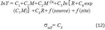
where Y is the ground motion parameter of interest, M the magnitude of the earthquake, R a measure of the distance from the source to the site being considered. C₁-C₉ are constants to be determined. The σ_lnY term describes the uncertainty in the value of the ground motion parameter given by the predicative relationship.

Regarding duration parameters many types of predictive relationships have been proposed (Bommer and Martinez-Pereira, 1999), but bracketed duration and significant duration relationships are the most commonly used. The former is defined as the time elapsed between the first and last excursions beyond a specified threshold acceleration. That definition has shown to be sensitive to the threshold acceleration considered and to small events that occur at the final part of a recording. Significant duration is based on the dissipation of energy, within a time interval, and this energy is represented by the integral of the square of the ground motions. In the case of acceleration is related to the Árias intensity IA (Árias, 1970):

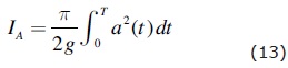
here a (t) is the acceleration time history, g is the acceleration of gravity, and T represents the complete duration of recording a (t). Figure 5 present the procedure followed to determine the significant parameters (Husid, 1969). The most common measure of significant duration is a time interval between 5-95% of IA and is denoted by D_a5-95.

Predictive relationships have also been developed for frequency-dependent duration parameters evaluated from bandpassed accelerograms (e.g., Bolt, 1973, Trifunac and Westermo, 1982; Mohraz and Peng, 1989; and Novikova and Trifunac, 1994). These relationships have several limitations that are basically associated with a deficient representation of magnitude or site effects. Additionally, none of these have been derived from the energy integral. Some other restrictions are related to measured distan-ce (normally the epicentral distance, not the closest site-source distance) and finally there are still others having to do with the regression method used to derive the relationships (Kempton and Stewart, 2006).

In what follows we develop a predictive neuronal model for significant duration that: 1) considers the seismic effects associated to magnitude, focal distance, near-fault rupture directivity and soil conditions and 2) is based on a soft computing procedure that accounts for inter- and intra-event ground-motion variability. Significant duration, from the Árias integral, was selected because of the stability of the method with respect to the definitions of initial and final threshold (Bommer and Martinez-Pereira 1999).

 

Neural estimation of duration

The ground motion duration model developed here captures the effects of the amount of energy radiated at the source using a neural representation of phenomena implicit in the data, the attenuation of seismic waves along the path due to geometric spreading and energy absorption; it also considers a local modification of the seismic waves as they traverse near-surface materials. The strong-motion duration D is the dependent variable of the NN formulation. The primary predictor variables (independent variables in a typical regression analysis) are M moment magnitude; R epicentral distance; focal depth FD, soil characterization expressed by Ts natural period; and Az azimuth.

 

NN based on information compiled from Puebla

Database

The city of Puebla has currently an accelerograph network composed of 11 seismic stations, three of which are located on rock, seven on compressible soil, and one in the basement of a structure. The general characteristics are provided in Table 1 and their locations indicated in Figure 6. Although, the first station (SXPU) was installed in 1972, the number of accelerogram records is relatively low mainly due to the low rate of seismicity in the region and the long process taken to install seismic stations.

In the first stage for the integration of our database, records with low signal-to-noise ratios were not taken into account. Hence, only 42 three-component accelerograms associated to three seismic stations (PBPP, SXPU and SRPU) are included in the database. These records were obtained from records of both subduction and normal-faulting earthquakes, originated, respectively, at the contact of the North America and Cocos plates, and by the fracture of the subducted Cocos plate.

The earthquakes in the database have magnitudes ranging from 4.1 to 8.1. Most of the events originated along coast of the Pacific Ocean in the states of Michoacan, Guerrero and Oaxaca. The epicenters of the remaining three events, those of October 24, 1980, April 3, 1997 and June15, 1999 were located in the Puebla-Oaxaca border. Epicentral distances to stations in the city of Puebla range from 300 to 500 km and in only one case it reached 800 km. That is why accelerations produced by the earthquakes considered in this research did not exceed 10 gal in Puebla.

In a second stage the database was expanded with accelerograms from the Instituto de Ingeniería UNAM Accelerographic Network (Alcántara et al., 2000). The added acceleration histories were recorded in stations on rock located the coastal region of the states of Michoacan, Guerrero and Oaxaca, and forcefully had to be generated by one of the earthquakes we had already catalogued in Table 1. The seismic stations we considered are shown in Figure 7 (filled squares), as well as the locations of the epicenters (inverted triangles). They were 88 three-component accelerograms in the final database.

A set of 26 events was used (Table 2) to design the topology of the NNs. These events were selected on the basis of the quality and resolution of the records. Accelerograms with low signal to noise ratios were deleted from the database. Both horizontal components and vertical direction of each seismic event were considered.

It is clear that the inputs and output spaces are not completely defined; the phenomena knowledge and monitoring process contain fuzzy stages and noisy sources. Many authors have highlighted the danger of inferring a process law using a model constructed from noisy data (Jones et al., 2007). It is imperative we draw a distinction between the subject of this investigation and that of discovering a process from records. The main characteristic of NN model is unrevealed functional forms. The NN data-driven system is a black-box representation that has been found exceedingly useful in seismic issues but the natural principle that explains the underlying processes remains cryptic. Many efforts have been developed to examine the input/output relationships in a numerical data-set in order to improve the NN modeling capabilities, for example Gamma test (Kemp et al., 2005; Jones et al., 2007; Evans and Jones, 2002), but as far as the authors' experience, none of these attempts are applicable to the high dimension of the seismic phenomena or the extremely complex neural models for predicting seismic attributes.

 

Neural approximation

The first step in developing a NN is the representation of the set of input and output cells. There are no clear-cut procedures to define this construction step. While the optimum architecture --hidden nodes and associated weights-- is obtained when the error function is minimized (i.e., the sum of the patterns of the squared differences between the actual and desired outputs is minimum) the numerical or categorical representation of inputs and outputs also depends on the modeler's experience and knowledge and a trial-and-error procedure must be followed in order to achieve a suitable design.

The RACP database has been modeled using the BP learning algorithm and Feed Forward Multilayer architecture. Time duration in horizontal (mutually orthogonal D_H1, N-S, and D_H2, E-W) and vertical components (D_V) are included as outputs for neural mapping and this attempt was conducted using five inputs (M, R, F_D, T_s and A_Z). After trying many topologies, we found out that the best model during the training and testing stages has two hidden layers with 200 nodes each. As seen in Figure 8a, the training correlation for D_H1, D_H2 and D_V was quite good, but when the same model is tested (unseen cases are presented to predict the output) considerable differences between measured and estimated duration times are found (Figure 8b). It is important to point out that the results shown in that figure are the best we were able to obtain after trying 25 different topologies. Thus, this can be considered as the model having the best generalization capabilities using the selected learning algorithm, architecture, and nodal hidden structure. In Figure 9 the estimated values obtained for a second set of unseen patterns (validation set) are compared with the numerical predictions obtained using the relationship proposed by Reinoso and Ordaz (2001). The neuronal relationship follows more narrowly the overall trend but fails in some cases, (coefficients of correlation around R²=0.75). It should be stressed that the NN has better interpolation and extrapolation capabilities than the traditional functional approaches. Furthermore, the influence of directivity and fault mechanism on duration can be identified with the NN, based on a multidimensional environment (Figure 10)

 

NN based on information compiled from Oaxaca

Database

The information used in the study is taken from the Oaxaca accelerographic array (RACO, Red Acelerográfica de la Ciudad de Oaxaca, in Spanish). The first recording station was installed in 1970 and nowadays the network comprises seven stations deployed around the urban area.

The instruments in these stations are located on ground surface. Each station has a digital strong-motion seismograph (i.e., accelerograph) with a wide frequency-band and wide dynamic range. Soil conditions at the stations vary from soft compressible clays to very stiff deposits (see Table 3). Locations of these observation sites are shown in Figure 11. From 1973 to 2004, the network recorded 171 time series from 67 earthquakes with magnitudes varying from 4.1 to 7.8 (Table 4). Events with poorly defined magnitude or focal mechanism, as well as records for which site-source distances are inadequately constrained, or records for which problems were detected with one or more components were removed from the data sets. The final training/testing set contains 147 three-component accelerograms that were recorded in five accelerograph stations OXLC, OXFM, OXAL, OXPM and OXTO. This catalogue represents wide-ranging values of directivity, epicentral distances and soil-type conditions (see Figure 12).

Neural modeling

The NN for Oaxaca City was developed using a similar set of independent parameters as those used for Puebla exercise. As the input/output behavior of the previous system is physical meaning the same five descriptors are included as inputs. This action permits to explore both systems' behaviors and to get wide-ranging conclusions about these variables.

Epicentral distance R was selected as a measure of distance because simple source-site relationships can be derived with it. Focal depth FD, was introduced for identifying data from interface events (FD < 50 km) and intraslab events (FD > 50 km). Together with the Azimuth Az, it associates the epicenter with a particular seismogenic zone and directivity pattern (fault mechanism).

To start the neuro training process using the Oaxaca database Ts is disabled and a new soil classification is introduced. Three soil classes were selected: rock, alluvium and clay. The final topology for RACO data contains BP as the learning algorithm and Feed Forward Multilayer as the architecture. Again D_H1, D_H2, and D_V are included as outputs for neural mapping and between the five inputs, four are numerical (M, R, F_D, and A_Z) and one is a class node (soil type S_T). The best model during the training and testing stages has two hidden layers of 150 nodes each and was found through an exhaustive trial and error process.

The results of the RACO NN are summarized in Figure 13. These graphs show the predicting capabilities of the neural system comparing the task-D values with those obtained during the NN training phase. It can be observed that the durations estimated with the NN match quite well calculated values throughout the full distance and magnitude ranges for the seismogenic zones considered in this study. Duration times from events separated to be used as testing patterns are presented and compared with the neuronal blind evaluations in Figure 14. The results are very consistent and remarkably better than those obtained when analyzing RACP database. The linguistic expression of soil type is obviously a superior representation of the soil effect on D prediction.

A sensitivity study for the input variables was conducted for the three neuronal modules. The results are given in Figure 15 and are valid only for the data base utilized. Nevertheless, after conducting several sensitivity analyses changing the database composition, it was found that the RACO trend prevails: S_T (soil type) is the most relevant parameter (has the larger relevance), followed by azimuth Az, whereas M, F_D and R turned out to be less influential. NNs for the horizontal and vertical components are complex topologies that assign nearly the same weights to the three input variables that describe the event, but an important conclusion is that the material type in the deposit and the seismogenic zone are very relevant to define D. This finding can be explained if we conceptualize the soil deposit as a system with particular stiffness and damping characteristics that determine how will the soil column vibrate and for how long, as seismic waves traverse it and after their passage through the deposit.

Through the {M, R, F_D, A_Z, S_T} → {D_H1, D_H2, D_V} mapping, the neuronal approach we presented offers the flexibility to fit arbitrarily complex trends in magnitude and distance dependence and to recognize and select among the tradeoffs that are present in fitting the observed parameters within the range of variables present in data.

 

Conclusions

Artificial neural networks were used to estimate strong ground motion duration. These networks were developed using a back propagation algorithm and multi-layer feed-forward architecture in the training stage. In developing the networks it was assumed that the parameters that have the greatest influence on strong motion duration are magnitude, epicentral distance, focal depth, soil characterization and azimuth. These parameters include the effects of seismic source, distance, materials and directivity. The many topologies tested and the input sensitivity developed drive to the conclusion that a broad soil-type classification (in these investigation three soil types) provides a better correlation with seismic phenomena than the more commonly used natural period T_s.

Overall, the results presented here show that artificial neural networks provide good and reasonable estimates of strong ground motion duration in each one of the three orthogonal components of the accelerograms recorded in the cities of Puebla and Oaxaca using easy-to-obtain input parameters: S M, R, F_D and A_z.

Finally, it is important to highlight that the capabilities of a NN ultimately depend on various factors that require the knowledge of the user about the problem under consideration. This knowledge is essential for establishing the pattern parameters that best represent it. Experience to set and to select the network architecture (including learning rules, transfer functions and hidden nodal structure) and the proper integration of training, test and validation data sets are also very important.

 

Acknowledgments

The recordings used in this paper were obtained thanks to Instituto de Ingeniería, UNAM and the Benemérita Universidad Autónoma of Puebla (BUAP). We are also grateful to Professor Miguel P Romo for his useful comments.

 

References

Adalbjörn S., Končar N., Jones A.J., 1997, A note on the Gamma test. Neural Computing and Applications, 5, 3, 131-133.         [ Links ]

Alcántara L., González G., Almora D., Posada-Sánchez A.E., Torres M., 1999, Puebla City Accelerograph Network, activities in 1996, RACP-II/BUAP-01. Internal Report Institute of Engineering, UNAM and Autonomous University of Puebla, México, April (in Spanish).         [ Links ]

Alcántara L., Quaas R., Pérez C., Ayala M., Macías M.A., Sandoval H., (II-UNAM), Javier C., Mena E., Andrade E., González F., Rodríguez E., (CFE), Vidal A., Munguía L., Luna M.,(CICESE), Espinosa J.M., Cuellar A., Camarillo L., Ramos S., Sánchez M., (CIRES), Quaas R., Guevara E., Flores J.A., López B., Ruiz R., (CENAPRED), Guevara E., Pacheco J., (IG-UNAM), Ramírez M., Aguilar J., Juárez J., Vera R., Gama A., Cruz R., Hurtado F., M. del Campo R., Vera F., (RIIS), Alcántara L. (SMIS), 2000, Mexican Strong Motion Data Base, CD Rom Vol 2. Mexican Society for Earthquake Engineering.         [ Links ]

Anderson J.G., 2004, Quantitative measure of goodness-of-fit of synthetic seismograms, in 13th World Conference on Earthquake Engineering, 243, Vancouver, Canada, 1-6 August.         [ Links ]

Árias A., 1970, A measure of earthquake intensity, Seismic Design of Nuclear Power Plants. R. Hansen, Editor, MIT Press, Cambridge, Mass., 438-483.         [ Links ]

Bishop C.M., 1996, Neural networks for pattern recognition. Oxford University Press, New York, 482 pp.         [ Links ]

Bolt B.A., 1973, Duration of strong ground motion, in 5th World Conference on Earthquake Engineering, 292, Rome, Italy, 25-29 June.         [ Links ]

Bommer J.J., Martinez-Pereira A., 1996, The prediction of strong-motion duration for engineering design, in 11th World Conference on Earthquake Engineering, 84, Acapulco, Mexico, 23-28 June.         [ Links ]

Bommer J.J., Martinez-Pereira A., 1999, The effective duration of earthquake strong motion. Journal of Earthquake Engineering, 3:2, 127–172.         [ Links ]

Broomhead D.S., Lowe D., 1988, Multivariable functional interpolation and adaptive networks, Complex Systems, 2, 321-355.         [ Links ]

Evans D., Jones A.J., 2002, A proof of the Gamma test. Proc. R. Soc. Lond., 458, 2759-2799.         [ Links ]

Hassoun M.H., 1995, Fundamentals of Artificial Neural Networks. MIT Press, Massachusetts, 511 pp.         [ Links ]

Hertz J., Krogh A., Palmer R.G., 1991, Introduction to the Theory of Neural Computing. Addison-Wesley, California, 327 pp.         [ Links ]

Jones A.J., Evans D., Kemp S.E., 2007, A note on the Gamma test analysis of noisy input/output data and noisy time series. Physica D, 229:1, 1-8.         [ Links ]

Tettamanzi A., Tomassini M., 2001, Soft Computing: integrating evolutionary, neural, and fuzzy systems. Springer-Verlag, Berlin, 328 pp.         [ Links ]

Husid L.R., 1969, Características de terremotos - análisis general. Revista del IDIEM, 8, 21–42.         [ Links ]

Kemp S.E., Wilson I.D., Ware J.A., 2005, A tutorial on the Gamma test. International Journal of Simulation: Systems, Science and Technology, 6:1-2, 67-75.         [ Links ]

Kempton J., Stewart J., 2006, Prediction equations for significant duration of earthquake ground motions considering site and near-source effects. Earthquake Spectra, 22:4, 985–1013.         [ Links ]

Mohraz B., Peng M.H., 1989, The use of low-pass filtering in determining the duration of strong ground motion. Publication PVP-182, Pressure Vessels and Piping Division, ASME, 197–200.         [ Links ]

Novikova E.I., Trifunac, M.D., 1994, Duration of strong ground motion in terms of earthquake magnitude, epicentral distance, site conditions and site geometry. Earthquake Eng. Struct. Dyn., 23, 1023–1043.         [ Links ]

Reinoso E., Ordaz M., 2001, Duration of strong ground motion during Mexican earthquakes in terms of magnitude, distance to the rupture area and dominant site period. Earthquake Eng. Struct. Dyn, 30, 653-673.         [ Links ]

Sarma S.K., 1970, Energy flux of strong earthquakes. Tectonophysics, 11, 159–173.         [ Links ]

Trifunac M.D., Westermo B.D., 1982, Duration of strong earthquake shaking. Soil Dynamics and Earthquake Engineering, 1:3, 117-121.         [ Links ]