Original paper

 

Parallel numerical simulation of two-phase flow model in porous media using distributed and shared memory architectures

 

Luis Miguel de la Cruz* and Daniel Monsivais

 

Instituto de Geofísica, Departamento de Recursos Naturales, Universidad Nacional Autónoma de México, Ciudad Universitaria, Delegación Coyoacán, 04510 Mexico D.F., México. *Corresponding author: luiggix@gmail.com

 

Received: October 10, 2012.
Accepted: May 03, 2013.
Published on line: December 11, 2013.

 

Resumen

En este trabajo se estudia un modelo de flujo bifásico (agua-aceite) en un medio poroso homogéneo considerando un desplazamiento inmiscible e incompresible. Este modelo se resuelve numéricamente usando el Método de Volumen Finito (FVM) y se comparan cuatro esquemas numéricos para la aproximación de los flujos en las caras de los volúmenes discretos. Se describe brevemente cómo obtener los modelos matemático y computacional aplicando la formulación axiomática y programación genérica. También, implementa dos estrategias de paralelización para reducir el tiempo de ejecución. Se utilizan arquitecturas de memoria distribuida (clusters de CPUs) y memoria compartida (Tarjetas gráficas GPUs). Finalmente se realiza una comparación del desempeño de estas dos arquitecturas junto con un análisis de los cuatro esquemas numéricos para un patrón de flujo de inyección de agua, con un pozo inyector y cuatro pozos productores (five-spot pattern).

Palabras clave: flujo bifásico, medios porosos, recuperación de hidrocarburos, método de volumen finito, cómputo paralelo, Cuda.

 

Abstract

A two-phase (water and oil) flow model in a homogeneous porous media is studied, considering immiscible and incompressible displacement. This model is numerically solved using the Finite Volume Method (FVM) and we compare four numerical schemes for the approximation of fluxes on the faces of the discrete volumes. We describe briefly how to obtain the mathematical and computational models applying axiomatic formulations and generic programming. Two strategies of parallelization are implemented in order to reduce the execution time. We study distributed (cluster of CPUs) and shared (Graphics Processing Units) memory architectures. A performance comparison of these two architectures is done along with an analysis of the four numerical schemes, for a water-flooding five-spot pattern model.

Key words: two phase flow, porous media, oil recovery, finite volume method, parallel computing, Cuda.

 

Introduction

New recovery techniques (for example Enhanced Oil Recovery) are essential for exploiting efficiently oil reservoirs existing around the world. However, before these techniques can be successful applied, it is fundamental to develop mathematical and computational investigations to model correctly all the processes that can occur. General procedures for constructing these mathematical and computational models (MCM) are presented in [1, 2], where it is shown that with an axiomatic formulation it is possible to achieve generality, simplicity and clarity, independently of the complexity of the system to be modeled. Once we have an MCM of the oil recovery process we are interested in, an efficient implementation of computer codes is required to obtain the numerical solution in short times.

Nowadays, the oil reservoir characterization technologies can produce several millions of data, in such a way that an accurate well-resolved simulation requires an increase on the number of cells for the simulation grid. The direct consequence is that the calculations are significantly slow down, and a very high amount of computer resources (memory and CPU) are needed. Currently, fast simulations on commercial software are based on parallel computing on CPU cores using MPI [3] and OpenMP [4]. On the other hand, since the introduction of the CUDA language [5], high-performance parallel computing based on GPUs has been applied in computational fluid dynamics [6, 7], molecular dynamics [8], linear algebra [9, 10], Geosciences [11], and multi-phase flow in porous media [12, 13, 14, 15, 16] among many others.

The water-flooding technique is considered as a secondary recovery process, in which water is injected into some wells to maintain the field pressure and to push the oil to production wells. When the oil phase is above the bubble pressure point, the flow is two phase immiscible and there is no exchange between the phases, see [17]. Otherwise, when the pressure drops below the bubble pressure point, the hydrocarbon component separates into oil and gas phases. The understanding of the immiscible water-flooding technique is very important and still being studied as a primary benchmark for new numerical methods [18] and theoretical studies [19]. Besides, some authors have started to investigate parallel technologies to reduce the execution time of water-flooding simulations, see for example [7, 13, 15, 20].

The incorporation of the GPUs into the floating point calculation of the oil reservoir simulation, has been considered in several studies. For example, in [20] a model for two-phase, incompressible, immiscible displacement in heterogeneous porous media was studied, where an operator splitting technique, and central schemes are implemented on GPUs producing 50-65 of speedup compared with Intel Xeon Processors. In [13], a very similar study as ours is presented, where the IMPES method is used to linearize and decouple the pressure-saturations equation system, and the SOR method is applied to solve the pressure equation implicitly. Their implementations was done considering a partition of the domain and then distributing each subdomain to blocks of threads. They obtain considerable accelerations (from 25 to 60.4 times) of water-flooding calculations in comparison with CPU codes. Multi-GPU-based double-precision solver for the three-dimensional two-phase incompressible Navier-Stokes equations is presented in [7]. Here the interaction of two fluids are simulated based on a level-set approach, high-order finite difference schemes and Chorin's projection method. They present an speed-up of the order of three by comparing equally priced GPUs and CPUs.

The numerical application studied in this paper, is the well known five-spot pattern model, and we work this model in the limit of vanishing capillary pressure, applying Darcy's law coupled to the Buckley-Leverett equation. This assumption generates an hyperbolic partial differential equation which can presents shocks in its solution. Our approach for solving this equation is to use four numerical schemes for approximating the fluxes adequately on the faces of the discrete volumes. We are interested in to study the numerical throwput of these four numerical schemes. We also focus our attention in the comparison of two parallel implementations written to run on a high-performance architecture consisting of CPUs and GPUs. We made this comparison in equality of conditions in order to do an objective analysis of the performance. The parallel implementations we present, are based on the use of well established opensource numerical libraries for solving linear systems. We use PETSc [21, 22] for distributed memory and CUSPARSE [24, 23] for GPU shared memory. We coupled these two libraries to our software TUNAM [25, 26], which implements FVM from a generic point of view. With this software we can easily implement, incorporate and evaluate the four numerical schemes for the approximation of the fluxes on the faces. Our objective is to give a quantitative reference that can be reproduced easily, and applied to other applications.

This paper is structured as follows. In section 2, we discuss the mathematical modeling of multiphase flows in porous media. The presentation is based on the axiomatic formulation introduced in [1, 2], and a pressure-saturation formulation is described for the two-phase flow. In section 3, the FVM is applied to the mathematical model, and the four numerical schemes for approximating the fluxes on the faces are introduced. We also explain the IMPES method used to obtain the solutions. The computational implementation of the algorithms, including our parallel implementations are also explained. In section 4, we solve the five-spot model using the four numerical schemes in combination with a linear and quadratic relative permeability models. In section 5, an analysis of the performance of our parallel implementations is done. Finally, in section 6 we give our conclusions.

 

Governing equations of a multiphase system

Given an intensive property ψ and a reference body B(t) of a continuous system, the general balance equation, in conservative form see [27], can be written as follows

where x represents the position and t is the time. In equation (1) the flux function is defined as F =vψ—τ, and the quantities v(x, t), q(x, t) and t(x, t) represent the velocity of the particles of B(t), the generation and the flux of property ψ, respectively (see [1] for a complete description on this formulation).

In a multiphase porous media system, the mass of fluid of the phase α is an extensive property M_α, and the corresponding intensive property is ψ_α. Both properties are related as follows

where the intensive property is defined as ψ_α = Φρ_αS_α. Here f is the porosity, ρ_α and S_α are the density and the saturation of phase respectively.

From equation (1), and using the fact that B(t) is arbitrarily chosen, the conservative form of the balance equation for the mass of fluid of the phase α is

where the flux function F_α is defined as

In equation (3) we have introduced the Darcy's law for multiphase systems

where λ_α is the mobility of the phase α defined as λ_α=k_rα/µ_α. Here k_rα is the relative permeability of phase α. The viscosity, the pressure and the density of phase α are denoted by µ_α, p_α and ρ_α, respectively. The tensor is the absolute permeability. The symbol ℘ is the magnitude of earth gravity and represents the depth of the porous media, see [17]. We also used the Darcy's velocity of phase α defined as u_α=vΦS_α.

 

Pressure equation

Equation (2) represents a fully–coupled system of N_p phases. Using a pressure–saturation formulation, see [17], it is possible to decouple the N_p equations into one for a phase pressure and N_p−1 for saturations. These equations will be weakly coupled and can be solved iteratively.

In order to obtain a pressure equation, we start from equation (2) and neglecting the diffusion τ_α = 0, dividing by ρ_α and summing over all phases, we obtain

Developing the derivatives and using the fact that we obtain the phase pressure equation

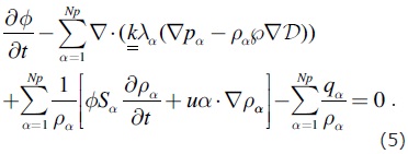
where the Darcy's law was written explicitly.

 

Saturation equation

The solution of equation (5) produce the pressure for a phase α. Other phase pressures can be obtained via the capillary pressure relations

where α₁ represent a non-wetting phase and α₂ represent a wetting phase.

Using the phase pressures we can calculate the velocities via Darcy's Law, equation (4). This velocity is necessary to solve the saturation equations (2), which can be written as follows

 

Incompressible two-phase pressure-saturation model

Two-phase flow in porous media modeling is concerned to the displacement of one fluid by another. In general, a wetting fluid, say water, is injected into the porous media displacing a non-wetting fluid, say oil, which is being extracted at another location. Due to the physical interaction between the two phases, this process generates a moving front at the interface between the phases. The evolution of the front is of primary interest for the production of hydrocarbons in oil recovery field.

We consider two incompressible and immiscible phases: water (w) and oil (o) in a porous media of constant porosity Φ. Equations are commonly posed in terms of the field variables oil pressure and water saturation as follows

where

and the source terms are defined as Q_w = q_w/ρ_w and Q_o = q_o/ρ_o. The capillary pressure is defined as p_cow(S_w) = p_o − p_w and because it depends on water saturation, it is possible to write ∇p_cow=(dp_cow/dS_w) ∇Sw. Equations (8) and (9) are coupled and non-linear. In order to decouple and linearize those equations, we employ the IMPES method, which will be explained in the next section. Note that equations (8) and (9) are simplified versions of equations (5) and (7), respectively.

 

Numerical model

The numerical formulation of the equations (8) and (9) is based on the finite volume method (FVM) which is derived on the basis of the integral form of the global balance equation (1), see [28, 29, 27].

In the FVM we keep track of an approximation to the integrals of equation (1) over each control volume, see figure 1. Every time step, we update these values using approximations to the fluxes throughout the faces of the volumes. When the approximations are calculated in a control volume, we transform the original equations into a set of algebraic equations.

Applying FVM to equation (8), and using the notation and we obtain the next discrete pressure equation

where the superscript is the time step and the subscripts indicate the node of the mesh according to figure 1. Equation (10) was obtained for a fully implicit temporal scheme and assuming that the aⁿ_NB coefficients, for NB∈{P, E, W, N, S, F, B}, can be calculated from values of the fluxes at instant n. The shape of aⁿ_NB coefficients depends on the numerical schemes used to approximate the fluxes on the control volume faces. In obtaining equation (10) we use the fact that the pressure equation is coupled with the saturation one, in such a way that, even though there is not temporal term in equation (8), we need to update the pressure field when a new saturation field is obtained.

The discretized form of equation (9) using FVM is

The shape of the coefficients for equations (10) and (11) are given in appendix A.

 

Numerical schemes for water saturation

Coefficients of equations (10) and (11) depends on the mobilities and capillary pressure evaluated on the faces of control volumes. These coefficients in turn depend on the water saturation, S_w, which is an unknown of the system of equations, and is updated every time iteration at the center of the volumes. In order to calculate the mobilities and the capillary pressure we require the value of S_w on the faces of volumes. There exist several approaches to evaluate S_w on the faces, and in this work we implemented four numerical schemes which are described below.

Upwind : linear upstream; for example for face e we have

Average : a weighted average is done using the neighbors to point P; for example for face e we have

UpwindE : quadratic upstream with extrapolation [30]; for example for face e we have

UpwindQ : cubic upstream [31]; for example for face e and uniform meshes we have

 

Solution method

The IMPES (IMplicit Pressure, Explicit Saturation) method is very used for solving two phase flow models of incompressible or slightly compressible fluids, see [17, 30]. As presented in sections §2.1 and §2.2, we can formulate our problem in terms of one equation for a phase pressure and N_p− 1 equations for phase saturations. In the IMPES method, for the two-phase case, we solve the pressure equation (8) implicitly and the saturation equation (9) explicitly. In order to solve the pressure equation, we use an initial saturation, and once the pressure is obtained, we can use it to solve the saturation equation. This process linearize and decouple the system of equations and is done iteratively for a given number of time steps. The IMPES method is given in algorithm (1).

Algorithm 1 IMPES

1: Initial data: S⁰, p⁰, T_max and Δt.

2: n ← 0.

3: while t < T_max do:

4: Calculate the coefficients of equation (10) using Sⁿ.

5: Solve discrete pressure equation (10) implicitly to obtain pⁿ.

6: Calculate the coefficients of equations (11) using pⁿ and Sⁿ.

7: Solve discrete saturation equation (11) explicitly to obtain Sⁿ⁺¹.

8: tⁿ⁺¹ ← tⁿ + Δt.

9: n ← n + 1.

10: end while

Even though that it is possible to use different time steps for pressure and saturation equations, here we use the same time step in order to evaluate the total elapsed time of pressure and saturation solution, when both are obtained for the same number of iterations.

 

Computational implementation

We use the software TUNAM [25] to implement the FVM applied to the equations described in previous sections. The TUNAM library use object-oriented and generic programming, in such a way that it is possible to extend its functionality to solve many sort of problems. In TUNAM there are three main concepts: Generalization, Specialization and Adaptors, which are related through the application in two levels of the Curiously Recurring Template Pattern [32].

The main generalization in TUNAM is the GeneralEquation concept, which refers to the general balance equation (1) and its FVM discrete formulation represented by equations (10) and (11). In principle, this general concept accounts for all the FVM coefficients. We inherit from this concept the TwoPhaseEquation, which is an specialization that includes all particular features of the two-phase model described in section §2.3. Because we are interested in to analyze the performance of the four numerical schemes described in section §3.1, we implement eight adaptors resumed in table 3.

Table 1

Next two lines of code explains how the pressure and saturation equations are defined in the TUNAM framework

TwoPhaseEquation<FSIP1<double, 3> > pressure(p, A, b, mesh);

TwoPhaseEquation<FSES1<double, 3> > saturation(Sw, A, b, mesh);

The pressure and saturation equations are defined in lines 1 and 2 of the above code, respectively. These equations are defined in terms of the objects p (pressure field), Sw (saturation field), A (matrix of algebraic system), b (source term) and mesh (mesh of the domain). The template parameters FSIP1 and FSES1 are two adaptors that define the shape of the coefficients of equations (10) and (11). We can use any of the adaptors listed in table 3, and the change in the code would be only in lines 1 and 2 (for example we can use FSIP2 and FSES2, instead). For more details of the TUNAM framework see [26].

Using the objects pressure and saturation the IMPES method is implemented in the next simple manner:

while (t <= Tmax) {
pressure.calcCoefficients();
Solver::TDMA3D(pressure, tol, maxIter);
pressure.update();
saturation.calcCoefficients();
Solver::solExplicit3D(saturation);
saturation.update();
t += dt;
}

 

Parallel implementation

Inside the IMPES algorithm (1), the step 5 is the most time consuming task. In the TUNAM code, related to the IMPES cycle as described in sections §3.2 and §3.3, the solution of the pressure equation can be achieved by different approaches. Due to the size of the problem, the use of iterative algorithms is usually the fast (and many times the only) way to get the solution vector. Among these, is the BiCGStab [33], a Krylov sub-space method, which gave us the better time convergence and stability than other similar methods. This solver method can be implemented easily in parallel exploiting different type of architectures. In this work, we study the performance of two memory architectures: a distributed memory of a cluster via the PETSc library[21, 22]; and a shared memory architecture of a Graphics Processing Unit (GPU) using the CUSPARSE library[24, 23], which is based on CUDA.

The linear algebra operations contained in a regular iteration of the BiCGStab method (without preconditioning) are listed in the table 1, as well as the number of times each operation is called inside the iteration. Using PETSc¹ and CUDA libraries we wrote down two codes with the same operations, as shown in table 1, in order to achieve the BiCGStab algorithm, see appendix B. Also, the same type of matrix's compression format was used to fix down the same conditions for both codes. In this case, the most time-consuming operations are the 2 matrix-vector product.

The Compressed Row Storage (CRS) format[34] was used to store the matrix of the linear system. In the CRS, the non-zero elements are stored in a linear array A*, and an auxiliary array J* is used to keep the column number j of each element of A*. In order to know the row of every element stored, a third array I* is used. This array keeps the segmentation of the array A* in elements of the same row in the original matrix , i.e. the position in the array A* of the first non-zero element of each row. For diagonal matrices, the growth in size of the data stored is O(n), against the O(n²) of the non-compressed counterpart.

We adapted the TUNAM code described in section §3.3 for using PETSc and CUDA. At the very beginning of each IMPES iteration, just after updating the matrix and vectors of the linear system for pressure, the containing arrays from TUNAM were handled to conform the format required by the two evaluated parallel libraries. The explicit solution of the saturation equation, can be expressed as a set of linear algebra operations (see appendix C). In this approach, the saturation vector S at time n + 1, is calculated as follows

where S, p, d, are vectors corresponding to equation (11) and , , are diagonal-banded matrices (see Appendix B) containing respectively, the coefficients bⁿ_NB, cⁿ_NB and dⁿ_NB. The linear operation (20) was translated to an equivalent parallel implementation, with 5 axpy's operations and 3 matrix-vector products.

 

Application to the five-spot pattern

Waterflooding is classified as a secondary oil recovery technique, which consists in the injection of water into the reservoir through injectors wells, pushing the hydrocarbons into the rocks and forced to flow towards the producers wells.

A simplified, but realistic two-phase flow model, is that from Buckley and Leverett [35], where we have two immiscible and incompressible fluids, the diffusivity and capillary pressure effects are ignored, and the gravity is neglected. With these considerations pressure equation (8) is elliptic, whilst saturation equation (9) is hyperbolic and may develop discontinuities in the solution. Applying the model of Buckley-Leverett, we studied the well established five-spot pattern. The domain of study is a parallelepiped domain, where four producers wells are located in the corners, and one injector well is in the center of the domain. Due to the symmetry only a quarter of the domain is simulated. The complete data set was taken from [18] and is resumed in table 2.

 

Relative permeability model

We use the Corey's model [36] to evaluate the relative permeabilities. This model is defined as follows

where the effective saturation is defined as S_e = (S_w − S_rw)/(1 −S_rw− S_ro).

Table 3 shows the adaptors implemented in TUNAM for this work, which combine the relative mobility model for and σ = 1, and 2 the numerical schemes presented in section §3.1.

 

Numerical results

Figures 2 and 3 show the distribution of water saturation after 600 days of simulation, for the cases lineal (σ = 1) and quadratic (σ = 2), respectively. The numerical schemes Upwind, Average, UpwindE and UpwindQ are presented in graphics (a), (b), (c) and (d) respectively of those figures. In the linear case, the water front is well behaved independently of the numerical scheme. Figure 4(a) presents the profiles of water saturation for the linear case, along a line joining the injector and extractor wells. We observe in this figure that all the four schemes are very similar; UpwindE scheme introduce a numerical diffusion, producing an smeared solution; the other three schemes approximate the water front more accurate, and the best is UpwindQ, which is O(Δx³). On the other hand, for the case σ = 2, figures 3(a) and (c) show similar distribution, while graphics (b) and (d) have a non-realistic behavior. This is more clear in figure 4(b). High-order schemes provide accurate approximation of the front, but when they are used in isolation will usually result in physically meaningless solutions. The situation arises from the violation of the so called "entropy condition", and to solve it a monotonicity constraint is required, see [37]. We do not address this problem in this work. The numerical scheme UpwindE produce the best solution for σ = 2.

 

Performance analysis

All the results presented in this section were obtained by executing our codes in a cluster with 216 (Intel(R) Xeon(R) CPU X5650 2.67GHz) cores. The interconnection between the nodes of the cluster is Gigabit Ethernet. Moreover, the cluster has a TESLA M4050 GPU, with 448 cuda cores. The parameters for the simulation were the same as those in the table 2. The number of volumes in the x, y, and z directions were 320, 320, and 16 respectively, given a total of 1638400 cells. We reach the memory limit of the GPU using this number of volumes.

 

Linear algebra operations

The most time-consuming linear algebra operations used inside the BiCGSTab (see table 1), for a fixed number of volumes, were evaluated. This evaluation gave us the optimal number of processors for using the PETSc library in our cluster. Using matrices and vectors of the same size, as those used in the whole two-phase simulation, a PETSc implementation of each linear algebra operation from table 1, was analyzed in terms of the average FLOPs (floating point operations per second) measured over 10000 executions, for a distinct number of cores (between 1 and 216). Next, the average FLOPs of same linear algebra operations for the CUSPARSE implementation were measured using the same parameters as with PETSc. The matrix-vector product, axpy operation, dot product and norm of a vector performances are shown respectively in graphics a), b), c) and d) of the figure 5. In all graphics, the results of the CUSPARSE operations are shown as a horizontal line (blue), because the number of cores is fixed in a GPU, giving us only one point to compare with. On the other hand, for the PETSc library it is possible to measure the FLOPs with several number of processor, and we have at most 216 in our cluster.

 

Convergence speed of the four numerical schemes

During the simulation, the evolution of the water front (shock) depends on the numerical scheme used to calculate the water saturation on the volume's faces, see section §3.1. The saturation field and each numerical scheme generates different conditions for the calculation of coefficients of discrete pressure equation. As a consequence, the linear system to be solved in the iterative process of the BiCGStab, will change its condition number depending particullarly on the numerical scheme. The profiles of the water front at a fixed time, using the four different numerical schemes described in section §3.1, was shown in the figure 4, where the scheme-dependence is clear. In order to take into account this dependence, in table 4 we show the average number of iterations done by the BiCGStab method to converge using a tolerance (relative error) of 10^-7, for each one of the four numerical schemes. We also report the condition number of the matrix generated by each one of the numerical schemes. The average is calculated over the total number of IMPES iterations (1200 steps) and a mesh of 80 x 80 x 4. The remaining data were the same as in table 2.

We observe from table 4 that the linear case, σ = 1, do not present any kind of complications, and the condition number and the average number of iterations is the same for all the four schemes. On the other hand, the case σ = 2 give us different numbers for different schemes. It can be observed that the best behaved scheme is the UpwindE, as we already observed in section §4.2.

We do not present the results for the case UpwindQ with σ = 2, because it was not able to converge. As we pointed out before, this implementation does not contains the monotonicity constrain and therefore the results are unrealistic for this case. Similar comments are valid for the Average with σ = 2, but in that case we do obtain convergence, although the numbers are not useful because it also presents a similar behavior as the UpwindQ scheme.

 

SpeedUp of the parallel IMPES method

The solving time for the pressure and saturation equations, during the simulation for PETSC and CUSPARSE are shown in the figure 6. We use non-dimensional time, defined as the ratio between the greater time (for one core in PETSc) between the times obtained for each number of cores. Again, the horizontal line (blue) represent the CUSPARSE result. Taking as reference the execution time with one core in the PETSc implementation, the speedup analysis is shown in the bottom graphic of the figure 6.

Here the speedup is defined as the ratio between the time taken to solve the pressure and saturation equations in a serial process, divided by the time taken in a parallel process (448 cores for CUDA and n cores for PETSc, with 1 ≤ n ≤ 192). All operations were executed with vector and matrices corresponding to a mesh of 1638400 nodes.

In figure 6 we observe that the best performance is obtained on the GPU for a fixed problem size. The speedup is almost 8 times in relation with the serial code. For the PETSc implementation, we observe that the peak performance is obtained for 12 processors. After that, the speedup starts to decrease monotonically as the number of processors is increased. This effect is due to the fact that the size of the problem is fixed and this size is tied to the memory of the GPU. When we increase the number of processor, the number of grid cells assigned to each processor by PETSc is reduced, and therefore, the communications between processors will have more impact on the execution time than the floating operations. We also recall that the interconnection of the cluster is not a high-end technology (for example infiniband), then is expected a reduction on the speedup when we increase the communications. Each node of our cluster contains 12 independent CPUs, which share memory. Hence, the results shown in figure 6 are compatible with the architecture of the cluster. Our conclusion here is that, in equality of conditions, a GPU TESLA M4050 GPU give us double of speedup than a node composed of 12 Intel Xeon processors, using CUSPARSE and PETSc as was described in the previous sections.

 

Conclusions

In this work we investigated the impact of four numerical schemes on the solution of a two-phase flow in an homogeneous porous media. Our study was focus on two objectives: 1) accuracy of the numerical scheme; and 2) performance in parallel using two memory architectures.

For the first objective, we found that the UpwindQ scheme, which is third order, gives the better approximation to the water-oil front than the other three, for the linear permeabilities model (σ = 1). In this case, all the schemes work fine, although some of them introduce numerical diffusion which smears the numerical solution. For the quadratic permeability model (σ = 2), it was observed that the best scheme was UpwindE, which is second order, and the Average and UpwindQ present unrealistic solutions due to the lack of a monotonicity constrain in their implementations. The Upwind scheme, which is first order, gives good approximation but produce higher numerical diffusion than UpwindE scheme.

The second objective was studied using two libraries: PETSc for distributed memory and CUSPARSE for GPUs where the memory is shared. We implemented a BiCGStab method with both libraries and we use similar operations in order to have equality of conditions. The saturation calculation step was implemented in terms of linear algebra operations, and we also measured the performance of this step. We obtained that, for a fixed problem size the CUSPARSE implementation is approximately two times the speedup than the PETSc one. At this point we can say that our CUSPARSE implementation for a single GPU, is a better option than our PETSc implementation executed on a 12 CPU node. On the other hand, the PETSc implementation can be used for a bigger problems size, and in the case of our cluster, we can run in at least 8 nodes, allowing to investigate eight times bigger problems. This is important for more realistic research were we have very large-scale data sets.

Finally, we can say that a GPUs cluster will have better performance than a CPU only cluster. In some cluster architectures it is possible to deploy more than one GPU by node, allowing more floating point operations powerful. Combining the CPU and GPUs, along with efficient opensour- ce libraries, like CUSPARSE and PETSc, we can face the challenge of oil reservoir simulation to a large-scale and more realistic formulations.

 

Acknowledgments

Luis M. de la Cruz wishes to acknowledge the support from the project IX10110 of DGAPA-UNAM to develop this research.

 

Bibliography

Aksnes E.O., 2009, Simulation of Fluid Flow Through Porous Rocks on Modern GPUs (Master degree thesis). Norwegian University of Science and Technology, Department of Computer and Information Science. http://ntnu.diva-portal.org/smash/record.jsf?pid=diva2:348910.         [ Links ]

Al-Huthali A., Datta-Gupta A., 2004, Streamline simulation of counter-current imbibition in naturally fractured reservoirs. Journal of Petroleum Science and Engineering, 43, 271–300.         [ Links ]

Amazianea B., Jurakb M., Kekoc A.G., 2011, An existence result for a coupled system modeling a fully equivalent global pressure formulation for immiscible compressible two-phaseflow in porous media, Journal of Differential Equations, 250, 3, 1685-1718.         [ Links ]

Anderson J., Lorenz C., Travesset A., 2008, General purpose molecular dynamics simulations fully implemented on Graphics Processing Units. Journal of Computational Physics, 227, 10, 5342-5359.         [ Links ]

Balay S., Brown J., Buschelman K., Gropp W.D., Kaushik D., Knepley M.G., Curfman McInnes L., Smith B.F., Zhang H., 2012, PETSc Web page, http://www.mcs.anl.gov/petsc.         [ Links ]

Balay S., Brown J., Buschelman K., Gropp W.D., Kaushik D., Knepley M.G., Curfman McInnes L., Smith B.F., Zhang H., 2012, PETSc Users Manual, ANL-95/11 - Revision 3.3, Argonne National Laboratory.         [ Links ]

Barrett R., Berry M., Chan T.F., Demmel J., Donato J., Dongarra J., Eijkhout V., Pozo R., Romine C., Van der Vorst H., 1994, Templates for the Solution of Linear Systems: Building Blocks for Iterative Methods, 2nd Edition, SIAM, Philadelphia, PA.         [ Links ]

Beisembetov I.K., Bekibaev T.T., Assilbekov B.K., Zhapbasbayev U.K., Kenzhaliev B.K., 2012, Application of GPU in the development of 3D hydrodynamics simulators for oil recovery prediction, AGH Drilling Oil Gas, 29, 1.         [ Links ]

Boris N. Chetverushkin B., Churbanova N.G., Morozov D.N., Trapeznikova M.A., 2010, Kinetic approach to simulation of multiphase porous media flow, V European Conference on Computational Fluid Dynamics ECCOMAS CFD 2010, J. C. F. Pereira and A. Sequeira (Eds), Lisbon, Portugal, 14-17.         [ Links ]

Buckley S., Leverett M., 1942, Mechanism of fluid displacement in sands. Trans. AIME, 146, 107–116.         [ Links ]

Bydal A., 2009, GPU-accelerated simulation of flow through a porous medium (Master degree thesis). Faculty of Engineering and Science, University of Agder, Grimstad May 25. http://brage.bibsys.no/hia/bitstream/URN:NBN:no-bibsys_brage_10942/1/Bydal.pdf.         [ Links ]

CUDA Toolkit 4.2, CUSPARSE Library NVIDIA Corporation, 2012, 2701 San Tomas Expressway, Santa Clara, CA 95050.         [ Links ]

Chen Z., Huan G., Ma Y., 2006, Computational Methods for Multiphase Flows in Poros Media, SIAM.         [ Links ]

Chen Z., 2007, Reservoir Simulation Mathematical Techniques in Oil Recovery, SIAM, Philadelphia, USA.         [ Links ]

Coplien J.O., 1995, Curiously recurring template patterns. C++ Report, 24–27.         [ Links ]

Corey A., 1954, The interrelation between gas and oil relative permeabilities. Prod. Montly, 19, 1, 38-41.         [ Links ]

Datta-Gupta A., King M.J., 2007. Streamline Simulation: Theory and Practice, Society of Petroleum Engineers Textbook Series Vol. 11.         [ Links ]

De la Cruz L.M., Template units for numerical applications and modelling (TUNAM) Web page, http://code.google.com/p/tunam/.         [ Links ]

De la Cruz L.M., Ramos E., 2012, General Template Units for the Finite Volume Method in Box-shaped Domains. Accepted to be published in Trans. Math. Soft.         [ Links ]

Herrera I., Pinder G.F., 2012, Mathematical Modeling in Science and Engineering: An Axiomatic Approach, John Wiley.         [ Links ]

Herrera I., Herrera G., 2010, Unified Formulation of Enhanced Oil-Recovery Methods, Geofisica Internacional, 2010.         [ Links ]

Kirk D.B., Hwu W., 2010, Programming Massively Parallel Processors: A Hands-on Approach (Applications of GPU Computing Series). Elsevier, Massachusetts.         [ Links ]

Leonard B.P., 1979, A stable and accurate conevctive modelling procedure based on quadratic upstream interpolation. Comp. Meth. in App. Mech. and Engineering, 19:59–98.         [ Links ]

Leveque R.J., 2004, Finite Volume Methods for Hyperbolic Problems. Cambridge University Press.         [ Links ]

Openmp: Simple, portable, scalable smp programming. http://www.openmp.org/.         [ Links ]

Patankar S.V., 1980, Numerical Heat Transfer and Fluid Flow. McGraw–Hill.         [ Links ]

Pereira F., Rahunanthan A., 2010, Numerical Simulation of Two-phase Flows on a GPU Proceedings of 9th International Meeting, High Performance Computing for Computational Science (VECPAR 2010), Berkeley, CA.         [ Links ]

Saad Y., 2000, Iterative Methods for Sparse Linear Systems. PWS/ITP 1996. Online: http://www-users.cs.umn.edu/~saad/books.html.         [ Links ]

Snir M., Otto S., Huss-Lederman S., Walker D., Dongarra J., 1998, MPI: The Complete Reference: Volume 1, The MPI Core. The MIT Press, Cambridge, Massachusetts, London, second edition edition.         [ Links ]

The NVIDIA CUDA Sparse Matrix library (cuSPARSE) Web page, 2012, http://developer.nvidia.com/cuda/cusparse.         [ Links ]

Tolke J., Krafczyk M., 2008, TeraFLOP computing on a desktop PC with GPUs for 3D CFD. International Journal of Computational Fluid Dynamics, 22, 7, 443-456.         [ Links ]

Tomova S., Dongarraa J., Baboulina M., 2010, Towards dense linear algebra for hybrid GPU accelerated many core systems. Parallel Computing, 36, 56, Pages 232-240.         [ Links ]

Torp A., 2009, Sparse linear algebra on a GPU with Applications to flow in porous Media (Master degree thesis). Norwegian University of Science and Technology, Department of Mathematical Sciences. http://ntnu.diva-portal.org/smash/record.jsf?pid=diva2:347855        [ Links ]

Trapeznikova M., Chetverushkin B., Churbanova N., Morozov D., 2012, Two-Phase Porous Media Flow Simulation on a Hybrid Cluster, I. Lirkov, S. Margenov, and J. Wasniewski (Eds.): LSSC 2011, LNCS 7116, pp. 646-653. Springer-Verlag Berlin Heidelberg.         [ Links ]

Versteeg H., Malalasekera W., 1995, An introduction to computational fluid dynamics: The finite volume method. Longman.         [ Links ]

Walsh S.D.C., Saar M.O., Bailey P., Lilja D.J., 2009, Accelerating geoscience and engineering system simulations on graphics hardware. Computers & Geosciences, 35, 2353-2364.         [ Links ]

Zaspel P., Griebel M., 2012, Solving incompressible two-phase flows on multi-GPU clusters. Computers & Fluids journal, In press.         [ Links ]

 

Nota

¹ Despite of PETSc has a biCGStab implementation, these includes operations not present in CUBLAS, as WAXPY.