Original paper

 

Use of Neural network to predict the peak ground accelerations and pseudo spectral accelerations for Mexican Inslab and Interplate Earthquakes

 

Adrián Pozos-Estrada¹*, Roberto Gómez² and H.P. Hong³

 

¹ Instituto de Ingeniería, Universidad Nacional Autónoma de México, Ciudad Universitaria, Delegación Coyoacán, 04510 México D.F., México. *Corresponding author: APozosE@iingen.unam.mx

² Instituto de Ingeniería, Universidad Nacional Autónoma de México, Ciudad Universitaria, Delegación Coyoacán, 04510 México D.F., México. E-mail: RGomezM@iingen.unam.mx

³ The University of Western Ontario, Department of Civil and Environmental Engineering, London, ON N6A 5B9, Canada. E-mail: hongh@eng.uwo.ca

 

Received: September 09, 2012.
Accepted: June 11, 2013.
Published on line: December 11, 2013.

 

Resumen

El uso de redes neuronales artificiales es explorado para predecir aceleraciones máximas del terreno y pseudoaceleraciones para sismos de tipo intraslab e interplaca. Un total de 277 y 418 registros sísmicos de dos componentes para sismos de intraslab e interplaca, respectivamente, son usados para entrenar los modelos de las redes neuronales artificiales con alimentación hacia adelante y con un algoritmo de aprendizaje de retroalimentación. Se consideran redes neuronales artificiales con una y dos capas ocultas. Con fines de comparación, valores de aceleración máxima del terreno y pseudoaceleración predichos con los modelos de las redes neuronales son comparados con los estimados mediante relaciones de atenuación o relaciones de movimiento fuerte. La comparación indica que los valores predichos, en general, siguen la tendencia de los valores obtenidos con las relaciones de movimiento fuerte. Sin embargo, se debe llevar a cabo una verificación extensa de los modelos entrenados antes que estos puedan emplearse en análisis de peligro y riesgo sísmico ya que, en ocasiones, los valores predichos no reflejan el comportamiento observado de los registros.

Palabras clave: red neuronal artificial, sismos de subducción, aceleración máxima del terreno, pseudoaceleración, México.

 

Abstract

The use of Artificial Neural Networks (ANN) is explored to predict peak ground accelerations (PGA) and pseudospectral acceleration (SA) for Mexican inslab and interplate earthquakes. A total of 277 and 418 seismic records with two horizontal components for inslab and interplate earthquakes, respectively, are used to train the ANN models by using an ANN with a feed-forward architecture with a back-propagation learning algorithm. Both ANN with single and two hidden layers are considered. For comparison purposes, the PGA and SA values predicted by the trained ANN models are compared with those estimated with attenuation relations or ground motion prediction equations (GMPEs). The comparison indicates that the predicted PGA and SA values by the trained ANN models, in general, follow the trends predicted by the GMPEs. However, an extensive verification of the trained models must be conducted before they can be used for seismic hazard and risk analysis since, on occasion, the PGA and SA values predicted by the trained ANN models depart from the behaviour observed from the actual records.

Key words: artificial neural network, subduction earthquakes, peak ground acceleration, pseudospectral acceleration, Mexico.

 

Introduction

Artificial neural networks (ANNs) have been used in seismic engineering due to their flexibility to deal with highly nonlinear problems (Fausett, 1994). ANNs have been used to predict ground motion measures such as the peak ground displacement (PGD), peak ground velocity (PGV), or peak ground acceleration (PGA), and spectral acceleration (SA) (Günaydin and Günaydin, 2008; Kamatchi et al., 2010). ANNs have also been used for generating artificial earthquakes and response spectra, and spectrum compatible accelerograms (Ghaboussi and Li, 1998; Lee and Han, 2002). More recently, Hong et al. (2012) showed that the prediction of the PGA and SA by using ANNs with a single hidden layer may not be robust, although it could be considered as an alternative to the commonly used attenuation relations or ground motion prediction equations (GMPEs). Estimation of PGAs for Mexican subduction earthquakes using the ANNs has been explored by García et al. (2007). However, the application of ANNs to predict SA for Mexican earthquakes has not been reported in the literature.

The main objective of this study is to investigate the applicability of ANNs to estimate PGA and SA for ground motion records caused by Mexican subduction earthquakes. Two sets of records of Mexican subduction earthquakes obtained at firm soil sites (i.e., site class B according to the NEHRP (BSSC, 2004)) are used in training and qualifying ANNs. Training of the ANN models was carried out using a feed-forward architecture with a back-propagation learning algorithm. Only single and two hidden layers are considered to minimize potential overfitting. The parameters considered in the input layer are: moment magnitude (M_w), closest distance to the fault (R_c) and focal depth (H), while the logarithm of the ground motion measures is used to represent the outcome from the output layer. The predicted PGA and SA values are compared with those estimated from GMPEs to assess the adequacy of the trained ANN models.

 

ANN Modeling

Description of the ANN modeling

The ANN modeling involves the selection of the number of neurons in the input as well as the hidden and output layers. In this study, the number of neurons in the input layer is considered to be 3, representing M_w, R_c and H as defined earlier. Single and two hidden layers (denoted by 1HL and 2HL, respectively) with multiple hidden neurons are used to approximate the mapping between the input and output layers. The output layer consists of a single neuron that represents the logarithm of the ground motion measures (PGA or SA) for a considered earthquake type and natural vibration period.

An illustration of an ANN model with multiple hidden layers and neurons is depicted in Figure 1, where neurons are weighted and transformed into output values. By considering two hidden layers, the mathematical expression of the output neuron in the output layer, y_output, is given by,

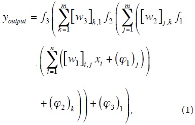
where n is the total number of neurons in the input layer; x_i is the i-th neuron in the input layer; [w₁]_{i, j}, [w₂]_{j, k} and [w₃]_{k, 1} are the weights that optimize the mapping between the input and the first hidden layer, between the first and second hidden layer and between the second hidden layer and output layer, respectively; (φ₁)_j, (φ₂)_k and (φ₃)₁ are the biases associated with the hidden and output layers; ƒ₁( ), ƒ₂( ) and ƒ₃( ) are activation (or transfer) functions between the input and the first hidden layer, the first and the second hidden layer and between the second hidden layer and the output layer, respectively; and m is the total number of neurons in the hidden layers.

Two types of activation functions, namely, the tan-sigmoid function and the linear function are commonly used. These functions are expressed as,

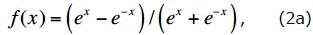
and

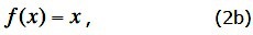
The former is often used as the transfer function between the input and hidden layers, while the latter is used as the transfer function between the hidden layers and the output layer. Following García et al. (2007), in the present study, Eq. (2a) is used as the transfer function between the input and hidden layer(s) and Eq. (2b) is used as the transfer function between the hidden layer(s) and the output layer.

 

Training ANN

The training of an ANN consists in the minimization of a predefined error function, in terms of observed and predicted output values, by varying the weights and biases. One of the algorithms used to train the ANN is the back-propagation (Fausset, 1994), where the error is propagated backward by adjusting the weights from the output to the input layer. The training can be summarized as follows:

1. Provide the ANN model with sample inputs and known outputs;

2. Evaluate an error function in terms of the difference between the predicted and observed output;

3. Minimize the error function by adjusting the weights and biases of all the layers from the output to the input layer.

For the numerical analysis to be presented in this study, the error function was defined as the mean square error (MSE). The minimization of the MSE (Step 3)) was carried out using the Levenberg-Marquardt algorithm (Marquardt, 1963; Press et al., 1992) that is incorporated into the back-propagation algorithm and implemented in Matlab (Hagan and Menhaj, 1994).

 

Strong ground motion database and GMPEs

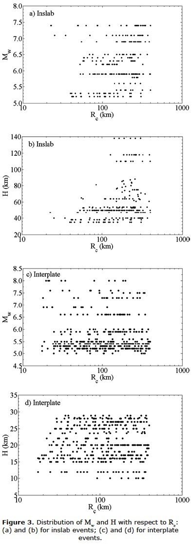
The strong ground motion database employed to develop the ANNs model consists of 695 strong ground motion records, each one with two horizontal components at firm soil sites (class B according to NEHNP –BSSC, 2004) complied by García et al. (2005, 2009). There are 277 inslab records and 418 interplate records for the events shown in Figure 2 and listed in Table 1. There are 16 intermediate-depth normal-faulting inslab events with M_w within 5.2 to 7.4 and 40 interplate events with M_w ranging from 5.0 to 8.0. The distribution of M_w and H with respect to R_c is presented in Figure 3. A baseline correction and a high-pass filter with cut-off frequencies of 0.05 Hz for events with Mw >6.5 and 0.1 Hz for the rest events were applied to all the records. The selection criteria of the records can be found in García et al. (2005, 2009). The same strong ground motion database was also employed by Hong et al. (2009) to develop GMPEs based on the geometric mean (i.e., for a random orientation). As these GMPEs will be used to compare with those predicted by the ANN model, the adopted functional forms and the obtained regression coefficients in Hong et al. (2009) are summarized below.

The functional form of the GMPEs for inslab earthquakes is the one given by García et al. (2005), which can be written as,

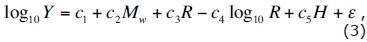
where Y (cm/s²) represents the PGA or SA values, c_i, i = 1, ..., 5, are the model parameters, M_w is the moment magnitude, 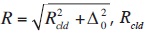(km) is the closest distance to the fault surface for events with M_w > 6.5, or the hypocentral distance for the rest, Δ = 0.0075 x 10^0.507Mw is a near-source saturation term defined by Atkinson and Boore (2003), H (km) is the focal depth, and ε is a zero mean error term with standard deviation σ, in which σ = (σ_r² + σ_e²)^0.5, and σ_r and σ_e denote the standard deviation due to intra- and inter-event variability, respectively. If the geometric mean for Y is considered, σ = (σ_r² + σ_e² + σ_c²)^0.5 and the standard deviation σ_c accounts for the random orientation variability.

For the records of interplate earthquakes, the functional form of the GMPE is the one employed by García (2006), which is expressed as,

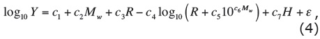
where c_i, i = 1, ..., 7, are the model parameters, R (km) is the closest distance to the fault surface for events with Mw > 6.0, or the hypocentral distance for the rest, and Y, M_w, H and e were defined previously. Note that in the above equation c₄ is considered to be given by the following equation (García 2006),

Using the adopted GMPEs, the records for the events detailed in Table 1, and the regression analysis algorithm given by Joyner and Boore (1993), Hong et al. (2009) obtained the model coefficients for a range of natural vibration periods based on the geometric mean. For an easy reference, the model coefficients for a few selected values of the natural vibration period, T_n, are presented in Tables 2 and 3. Moreover, for comparison purposes, the regression analysis in this study is carried out by considering either the first horizontal component (H1), or the second horizontal component (H2). The obtained model coefficients are also shown in Tables 2 and 3. As the H1 and H2 components represent the seismic excitation for a random orientation (with respect to the source), the developed model coefficients shown in Tables 2 and 3 will be used to predict PGA or SA for a random orientation.

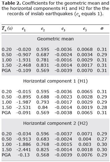
Comparison of the results shown in the tables indicates that the estimated model coefficients based on either only H1 or H2 components differ only slightly from those based on both components (i.e., geometric mean), as expected. Also, the average of the model coefficients obtained from H1 alone and from H2 alone is almost identical to those obtained based on the geometric mean. This fact simply confirms the robustness of the algorithm given by Joyner and Boore (1993) for developing the GMPEs. It also indicates that the number of records used for the purpose of regression analysis is adequate.

 

Prediction of strong ground motion measures using ANN

Effect of the number of hidden layers and neurons on the training ANN and on predicted values

The selection of the number of hidden layers and neurons is of importance in developing or training an ANN. This selection depends on the nature of the problem to be investigated, and a trial and error process is often followed to determine the adopted structure of the ANN model (Shahin et al., 2004). In selecting the ANN model, potential overfitting due to the use of an excessive number of hidden layers and/or neurons needs to be avoided, as this will lead to a lack of learning and the inability to predict the outcomes for scenarios not used in training. To avoid the possible overfitting, several preliminary ANN models were tested by considering combinations of the single and two hidden layers and up to 50 hidden neurons in each hidden layer. Furthermore, a total of 80% randomly selected records were used to train the model, while the remaining 20% of records were used for validating the trained model.

To investigate the effect of the record selection on the trained ANN model, a total of 300 trials were carried out. For each trial, a new set of PGA and SA values from 80% randomly selected records were used. For the analysis, only one component (H1 or H2) from each record is considered; both 1HL and 2HL models are employed for the training. As the results obtained for the H1 and H2 components from the records exhibit similar trend and the results for inslab and for interplate records are similar as well, we only illustrate the estimated MSE in Figure 4 for the H1 component from the inslab records.

Figure 4, which presents the results for PGA and SA at T_n = 1.5 s, shows scatter in the MSE. As expected, the scatter (but not necessarily the standard deviation) of the MSE increases as the number of trials increases. The average MSE estimated based on 300 trials, which is considered to be sufficient large, is illustrated in Figure 5 for the training stage. The results presented in this figure indicate that the lowest average MSE is obtained for n_n around 10, and that the average MSE is relatively consistent for the number of hidden neurons, n_n, up to 25. As the average MSE for n_n = 50 is much larger than that for n_n < 50, the use of n_n > 25 is not recommended.

By using the remaining 20% records to test the trained ANN models, the average of MSE for 300 trials was also calculated and presented in Figure 6. Comparison of Figures 5 and 6 indicates that average values of MSE for the trained ANN models shown in Figure 6 are slightly greater than those presented in Figure 5. This can be explained by noting that the trained ANN models are tested with input parameters that are different than those used during the training process. Figure 6 also shows that the use of the model with n_n = 50 leads to the greatest average MSE among the considered n_n values.

During the analysis, it was observed that the optimum number of neurons and hidden layers – those leading to the lowest MSE for the trained model – depend on the selected records. In all cases, the optimum number of neurons is within 3 to 20; in about 50% of time the 1HL model outperforms the 2HL model, and vice versa. To further inspect the differences of using the 1HL and 2HL ANN models, the mean of the ratio of the MSE of the trained 1HL model to that of the trained 2HL model shown in Figure 4 was calculated. The va-lues are presented in Table 4. The table indicates again that there is no clear preference among the 1HL and 2HL models, although the 1HL model for inslab earthquakes may be considered to perform better than the 2HL model. Based on these observations, the use of 10 neurons and the ANN model with 1HL and with 2HL will be considered in the next section.

 

Comparison of predictions using trained ANN

The training of the ANN models with 1HL and with 2HL was carried out by considering 10 neurons in each layer. For the analysis, the use of all H1 components and all H2 components are considered. As the results based on H1 or H2 components are almost the same, only the results for H1 are presented. Also, analysis was carried out by using only the geometric mean since this quantity is commonly used to develop GMPEs. For this case, the obtained weights and biases for the trained models are presented in the Appendix.

A comparison of the predicted PGA and SA by using the trained models to those obtained from the actual records is shown in Figures 7 and 8 for the H1 components and the geometric mean, respectively. It can be observed from the figures that there is a good agreement between the predicted and observed values, and that the correlation coefficient, ρ, is greater than 0.77 in all cases. The trained ANN models for inslab earthquakes provide better estimates than those for interplate earthquakes if H1 is considered; if the geometric mean is considered, both ANN models provide similar estimates. The scatter shown in the figures appears to be independent of the logarithm of PGA or logarithm of SA. A more detailed statistical investigation considering that the residual – η defined as the difference between the logarithmic of the actual PGA (or SA) and the logarithmic of the predicted PGA (or SA) – as a function of the predicted PGA (or SA) is beyond the scope of this study.

To provide a probabilistic characterization of the residual, η is shown in Figure 9 for a few selected cases presented in Figures 7 and 8. Inspection of the plots and use of a Kolmogorov-Smirnov test (Benjamin and Cornell, 1970) indicate that η can be modeled as a normal variable. The mean and the standard deviation of η for the cases presented in Figure 9 are summarized in Table 5, where the statistics of η, shown for the geometric mean case, were calculated by taking into account that the trained model will be used to predict ground motion measures for a random orientation, rather than the geometric mean (see Section 3).

 

Comparison of the predicted PGA and SA using trained ANN and GMPEs

To appreciate the adequacy of the trained ANN models for seismic hazard and risk assessment, a comparison of the trained models and the GMPEs is needed. The comparison is focused on the "average" behaviour and on the uncertainty in the model developed.

The uncertainty in the GMPEs is characterized by the statistics of ε (Tables 2 and 3), while that for the trained ANN is characterized by the statistics of the residual η (Table 5). A comparison of these tables indicates that although the trained ANN models are only slightly biased (i.e., the mean of h differs from zero), the degree of uncertainty in the trained ANN models, in terms of the standard deviation, is similar to that in the GMPEs. In parti-cular, the statistics of η and ε are very consistent for the case when the geometric mean was used to develop the GMPEs and to train the ANN models. Since η and ε shown in Eqs. (3) and (4) represent the difference between the logarithmic of the actual PGA (or SA) and the logarithm of the PGA (or SA) predicted by the ANN model and the GMPE, respectively, the physical meaning of η and ε is similar. η needs to be considered as an integral part of the developed ANN model if it is used for seismic hazard and risk analysis.

A comparison of the "average" behaviour of the trained ANN model and the GMPEs obtained, based on the geometric mean, is presented in Figures 10 and 11 for selected scenario events. It can be observed from these figures that in general the predicted values by the ANN model follow those predicted by the GMPEs. However, some differences are observed. The most pronounced are associated for R_c greater than 150 km. Moreover, in some cases, the predicted values by the trained ANN models may not necessarily reflect reality. For example, the results shown in Figure 10c indicate that SA can increase with distance beyond R_c = 200 km for M_w = 5.9 and H = 50 km, which is unrealistic. Since this drawback can be serious in engineering applications, tests of the trained ANN models must be conducted before they can be used to predict the ground motion measures for seismic hazard and risk assessments.

 

Conclusions

Artificial Neural Network models were developed to predict the ground motion measures for Mexican inslab and interplate earthquakes. The development used the PGA and SA calculated from single horizontal components of the records and from the geometric mean of the horizontal components. For training ANN model, the parameters for the input layer are moment magnitude, closest distance to the fault and focal depth, while the logarithmic of the PGA (or of the SA) is used to represent the outcome of the model. The main observations that can be drawn from the analysis results are:

1. The performance of the trained ANN model by using a single hidden layer is similar to that by using two hidden layers. The most appropriate number of neurons per hidden layer seems to be within 3 to 20.

2. The use of a single horizontal component or the geometric mean of the two horizontal components leads to similar trained ANN models, implying that the number of considered records is adequate.

3. The statistics of the residuals associated with the trained ANN models are similar to those associated with the GMPEs. The ground motion measures predicted by the trained ANN models follow those predicted by the GMPEs. This indicates that the ANN models may be a good alternative to GMPEs in some applications.

4. In some cases, the SA predicted by the trained ANN models increases as the R_c increases. This does not reflect the general behaviour observed from actual records. Therefore, extensive verification of the trained ANN models should be carried out before the models can be used for seismic engineering applications.

 

Acknowledgments

Financial support of the National Council of Science and Technology (CONACyT) of Mexico, the Natural Science and Engineering Research Council of Canada, the University of Western Ontario, and the IIUNAM are gratefully acknowledged. We thank T.J. Liu and S.C. Lee for many fruitful discussions, constructive comments and suggestions. We also thank two anonymous reviewers for their comments and suggestions that helped to improve this work.

 

Bibliography

Atkinson G.M., Boore D.M., 2003, Empirical ground-motion relations for subduction-zone earthquakes and their application to Cascadia and other regions. Bull. Seism. Soc. Am., 93, 1703-1729.         [ Links ]

BSSC, 2004, NEHRP Recommended provisions for seismic regulations for new buildings and other structures (FEMA 450), 2003 Edition.         [ Links ]

Benjamin J.R., Cornell C.A., 1970, Probability, Statistics and Decision for Civil Engineers. McGraw-Hill, New York.         [ Links ]

Fausset L.V., 1994, Fundamentals of neural networks: Architecture, algorithms, and applications. Prentice-Hall, Englewood Cliffs, N.J., 461 pp.         [ Links ]

García D., Singh S.K., Herraiz M., Ordaz M., Pacheco J.F., 2005, Inslab earthquakes of Central Mexico: Peak ground-motion parameters and response spectra, Bull. Seism. Soc. Am., 95, 2272-2282.         [ Links ]

García D., 2006, Estimación de parámetros del movimiento fuerte del suelo para terremotos interplaca e intraslab en México Central, PhD Tesis, Universidad Complutense de Madrid, Madrid, España. (In Spanish).         [ Links ]

García D., Singh S.K., Herraiz M., Ordaz M., Pacheco J.F., 2009, Erratum to Inslab Earthquakes of Central Mexico: Peak ground-motion parameters and response spectra, Bull. Seism. Soc. Am., 99, 2607-2609.         [ Links ]

García S.R., Romo M.P., Mayoral J.M., 2007, Estimation of peak ground accelerations for Mexican subduction zone earthquakes using neural networks. Geofisica Internacional, 46, 1, 51–63.         [ Links ]

Ghaboussi J., Li C.C.J., 1998, New method of generating spectrum compatible accelerograms using neural networks. Earthhquake Engineering and Structural Dynamics, 27, 4, 377–396.         [ Links ]

Günaydn K., Günaydn A., 2008, Peak ground acceleration prediction by artificial neural networks for northwestern Turkey. Mathematical Problems in Engineering, Art. No.: 919420.         [ Links ]

Hagan M.T., Menhaj M., 1994, Training feed-forward networks with the Marquardt algorithm. IEEE Transactions on Neural Networks 5, 6, 989-993.         [ Links ]

Hong H.P., Pozos-Estrada A., Gómez R., 2009, Orientation effect on ground motion measure for Mexican subduction earthquakes, Earthquake Engineering and Engineering Vibration, 8, 1, 1-16.         [ Links ]

Hong H.P., Liu T.J., Lee C.S., 2012, Observation on the application of artificial neural network for predicting ground motion measures. Earthq Sci., 25, 161–175.         [ Links ]

Joyner W.B., Boore D.M., 1993, Methods for regression analysis of strong-motion data. Bull. Seism. Soc. Am., 83, 469–487.         [ Links ]

Kamatchi P., Rajasankar J., Ramana G.V., Nagpal A.K., 2010, A neural network based methodology to predict site-specific spectral acceleration values. Earthq. Eng. & Eng. Vib., 9, 4, 459–472.         [ Links ]

Lee S.C., Han S.W., 2002, Neural-network-based models for generating artificial earthquakes and response spectra. Computers and Structures, 80, 1627–1638.         [ Links ]

Marquardt D.W., 1963, An algorithm for least squares estimation of non-linear parameters. Journal of the Society for Industrial and Applied Mathematics, 11, 2, 431-41.         [ Links ]

Press W.H., Teukolsky S.A., Vetterling A.W.T., Flannery B.P., 1992, Numerical Recipes in C: The Art of Scientific Computing. Cambridge University Press, New York.         [ Links ]

Shahin M., Maier H.R., Jaksa M.B., 2004, Data division for developing neural networks applied to geotechnical engineering. Journal of Computing in Civil Engineering, 18, 2, 105–114.         [ Links ]