Original paper

 

Relationship between solar radiation and dimethylsulfide concentrations using in situ data for the pristine region of the southern hemisphere

 

Jaime Osorio^1*, Blanca Mendoza² and Jorge Zavala-Hidalgo³

 

¹ Posgrado en Ciencias de la Tierra, Instituto de Geofísica, Universidad Nacional Autónoma de México. Circuito Exterior s/n, Ciudad Universitaria, Del. Coyoacán, 04510 México D.F., México. *Corresponding author: jaime@geofisica.unam.mx

² Departamento de Ciencias Espaciales, Instituto de Geofísica, Universidad Nacional Autónoma de México. Circuito Exterior s/n, Ciudad Universitaria Del. Coyoacán, 04510 México D.F., México.

³ Interacción Océano-Atmósfera, Centro de Ciencias de la Atmósfera, Universidad Nacional Autónoma de México. Circuito Exterior s/n, Ciudad Universitaria Del. Coyoacán, 04510 México D.F., México.

 

Received: September 10, 2012.
Accepted: January 09, 2013.
Published on line: September 30, 2013.

 

Resumen

Los procesos biológicos han sido propuestos como una de las componentes que hacen variar el clima. El Dimetilsulfuro (DMS) es el principal componente del sulfuro biogénico en la atmósfera. El DMS es producido, principalmente, por la biósfera marina y juega un papel importante en el ciclo del azufre atmosférico. Actualmente se acepta que la biota terrestre no sólo se adapta a las condiciones ambientales sino que las influencia a través de regulaciones en la composición química de la atmósfera. En este estudio se utiliza el método de ondeletas para investigar la relación entre DMS, Nubes bajas (LCC), Radiación Ultravioleta A (UVA), Radiación Solar Total (TSI) y Temperatura Superficial Oceánica (SST) en la llamada zona prístina del Hemisferio Sur. Se encontró que las series analizadas presentan diferentes periodicidades que pueden ser asociadas con fenómenos climáticos de gran escala tales como El Niño (ENSO) o la Oscilación Cuasi-Bienal (QBO), y/o con la actividad solar. Los resultados indican, de manera intermitente pero sostenida, una correlación DMS-SST y una anti-correlación DMS-UVA; pero DMS-TSI y DMS-LCC tienen una relación no lineal. La longitud temporal de las series sólo nos permite analizar periodicidades menores a 11 años, entonces, nos limitamos a analizar la posibilidad de que la radiación solar influya en el clima de la Tierra en periodos de tiempo menores que el ciclo solar de 11 años. Nuestros resultados también sugieren una interacción de retroalimentación positiva entre el DMS y la radiación solar.

Palabras clave: Dimetilsulfuro, Radiación Solar, clima, nubes, retroalimentación, análisis de Ondeleta.

 

Abstract

The biological processes have been proposed as climate variability contributors. Dimethylsulfide (DMS) is the main biogenic sulfur compound in the atmosphere; it is mainly produced by the marine biosphere and plays an important role in the atmospheric sulfur cycle. Currently it is accepted that terrestrial biota not only adapts to environmental conditions but also influences them through regulations of the chemical composition of the atmosphere. In the present study we used a wavelet method to investigate the relationship between DMS, Low cloud cover (LCC), Ultraviolet Radiation A (UVA), Total Solar Irradiance (TSI) and Sea Surface Temperature (SST) in the so called pristine zone of the Southern Hemisphere. We found that the series analyzed have different periodicities which can be associated with large scale climatic phenomena such as El Niño (ENSO) or the Quasi-Biennial Oscillation (QBO), and/or to solar activity. Our results show an intermittent but sustained DMS-SST correlation and a DMS-UVA anti correlation; but DMS-TSI and DMS-LCC show nonlinear relationships. The time-span of the series allow us to study only periodicities shorter than 11 years, then we limit our analysis to the possibility that solar radiation influences the Earth climate in periods shorter than the 11-year solar cycle. Our results also suggest a positive feedback interaction between DMS and solar radiation.

Key words: Dimethylsulfide, Solar Radiation, climate, clouds, feedback, wavelet analysis.

 

Introduction

The solar activity has been proposed as an external factor of Earth's climate change. Solar phenomena such as total and spectral solar irradiance could change the Earth's radiation balance and hence climate (Gray et al., 2010). However, biological processes have also been proposed as another factor of climate change through its impact on albedo associated with clouds. One of the most important issues regarding the Earth function system is whether the biota in the ocean responds to changes in climate (Charlson et al., 1987, Miller et al., 2003, Sarmiento et al., 2004). According to several authors, the major source of cloud condensation nuclei (CCN) over the oceans is dimethylsulfide (DMS) (e.g., Andreae and Crutzen, 1997; Vallina et al., 2007).

Dimethyl Sulphonium Propionate in phytoplankton cells is released into the water column where it is transformed into dimethylsulfide. The dimethylsulfide goes through the sea surface to the atmosphere as a gas, where it oxidizes to form a range of products, among them SO₂. This compound oxidizes to H₂SO₄, which forms sulphate particles that act as CCN. The dimethylsulfide concentration is controlled by the phytoplankton biomass and by a web of ecological and biogeochemical processes driving by the geophysical context (Simó, 2001). Solar radiation is the primary driving mechanism of the geophysical context and is responsible for the growth of the phytoplankton communities. Clouds have a major impact on the amount of heat and radiation budget of the atmosphere. Clouds modify both albedo (short-wave) and long-wave radiation. In particular, for low clouds over oceans, the albedo effect is the most important result of cloud radiation interaction and has a net cooling effect on the climate (Chen et al., 1999, Rossow, 1999).

The DMS, solar radiation and cloud albedo are hypothesized to have a feedback interaction (Charlson et al., 1987; Shaw et al., 1998; Gunson et al., 2006). This feedback can be either negative or positive. A negative feedback process requires a positive correlation between solar irradiance and DMS: increases in solar irradiance reaching the sea surface increase the DMS, augmenting the CCN and the albedo. An overall increase in the albedo produces a decrease in the irradiance reaching the sea surface and thus cooling occurs. A positive feedback requires an anti-correlation between solar irradiance and the DMS: decreases in solar irradiance produce a decrease of the DMS, the CCN and the albedo; a net reduced albedo allows more radiation to be absorbed, producing heating. Using seasonal and annual time scales, a first attempt to find correlations between a global database of DMS concentration and several geophysical parameters was unsuccessful (Kettle et al., 1999).

Quantitative studies that use data bases spanning roughly three decades (Simó and Dachs, 2002; Simó and Vallina, 2007; Vallina et al., 2007) have concluded that the DMS and solar radiation have a high positive correlation on seasonal time scales for most of the ocean, favoring a negative feedback on climate. Another study (Larsen, 2005), based on a conceptual model, proposed a positive feedback. A positive feedback would also imply an anti-correlation between Total Solar Irradiance (TSI) and cloud cover. Indeed, a global anti-correlation between TSI and oceanic low cloud cover has been found (Kristjánsson et al., 2002; Lockwood, 2005). Furthermore, case studies using ultraviolet (UV) light do not allow conclusive results regarding the sign of the solar radiation-DMS correlation (Kniventon et al., 2003; Toole and Siegel, 2004; Toole et al., 2006).

Another study on decadal relation between north and south high latitude concentrations of Methane Sulphonic Acid (MSA), associated exclusively to DMS, and TSI, found that at the time scales coincident with the 22-years magnetic solar cycle, the north-MSA and TSI follow each other, favoring a negative feedback on local climate; but at the time scales of the 11-years solar cycle for north and south, the MSA-TSI presents an anti-correlation that has increased since the 1940s favoring a positive feedback on local climate (Mendoza and Velasco, 2009), this indicates that the relations between the variables of interest may change with time and location.

The purpose of the present study is to examine in a selected location of the Southern Hemisphere and at time-scales shorter than the solar cycle the relationship between DMS and climate and DMS and solar phenomena, through clouds, sea surface temperature (SST) and the UV radiation A (UVA). A time series of UV radiation was used because this radiation has a role in a number of the key processes controlling DMS concentrations in seawater. Several studies link the production of DMS and UV (e.g. Toole et al., 2006, Kniventon et al., 2003), some studies report increases and other significant decreases in DMS production, also the phytoplankton responds dramatically to UV radiation (Toole and Siegel, 2004). These studies indicate a relationship between UV and DMS in the ocean (Kniventon, 2003).

 

Region of study and data

The data analysis was performed for the Southern Hemisphere between 40º- 75ºS latitude and 150W-155E longitude. Considering the abundance of chlorophyll by regions, this area includes the biogeochemical provinces ANTA, APLR, CHIL, FKLD, SANT and SSTC (Longhurst, 1995).

The concept of biogeochemical provinces is based on the observation that large ocean regions are characterized by coherent physical forcing and biological conditions at the seasonal scale, which are representative of macroscale ocean ecosystems. The boundaries between provinces are generally persistent but are also spatially and temporally variable, because they are linked to physical properties which are known to change position seasonally and inter annually. The boundaries of Longhurst's provinces were selected subjectively and intuitively on the basis of climatological data (mixed layer depth, solar irradiance penetration and chlorophyll concentrations) and common knowledge on the biological properties extracted from scattered data in the existing literature (Longhurst, 1995; Hardman-Mountford et al. 2008).

Longhurst (1995) recognize four primary domains of the global pelagic ecosystem. The first one is Polar: the seasonal cycle of sea ice in high latitudes results in a brackish surface layer in spring and summer as freshwater is released from melting winter ice cover; this phenomenon occurs most consistently in the marginal ice zone and leads to an active bloom as soon as ice break-up occurs). The second domain is Westerlies: the defining characteristic of this domain is seasonality in wind stress imposed by the westerlies associated with the Aleutian, Iceland and Antarctic atmospheric low-pressure cells, together with seasonality in the radiation flux at the sea surface. The third domain is Trade Winds: the Ekman layer of low latitudes is resistant to wind deepening and the scale of baroclinicity is weeks, rather than years as in higher latitude. The fourth domain is Coastal: the characteristic of this domain is to embrace the concept of a coastal boundary domain as defined for regions where the general oceanic circulation is significantly modified by interaction with coastal topography and with its coastal wind regimen.

These are themselves partitioned into 57 secondary biogeochemical provinces which we have used as the units of our global computation of primary production. For the Polar domain we use the biogeochemical provinces ANTA (Antarctic. Lies between the Polar Frontal Zone and the Antarctic Divergence, having two components: a zone of permanently open water and a zone seasonally carrying pack ice) and APLR (Austral Polar. This is a ribbon of westward-moving Antarctic Surface Water, up to 300 km wide, ice covered in winter but with some open water areas in summer, between the Antarctic Divergence and the continent). For the Westerlies domain we use the biogeochemical provinces SANT (Subantarctic. From the Subtropical Convergence south to the Antarctic Polar Front, which is the southern limit of the Polar Frontal zone and which covers ~4º latitude) and SSTC (South Subtropical Convergence. The most northerly of the annular features of the Southern Ocean. The frontal zone is sufficiently dynamic to have an associated eddy field and includes several surface discontinuity fronts). For the Coastal domain we use the biogeochemical provinces CHIL (Chile-Peru Current Coastal. Defined, like its Benguela homologue, as extending from the coastline to the offshore anticyclonic eddy field. To the south, it is defined by the divergence zone at ~45º S and to the north at its separation from the coast near the equator) and FKLD (Southwest Atlantic Continental Shelf. Argentine shelf and Falklands Plateau from Mar de Plata to Tierra del Fuego) (Longhurst, 1995).

This area (study region) is the least polluted in the world, the so-called pristine zone, and then solar effects on biota and climate should be more evident. Over 90% of the area is ocean; the remaining 10% corresponds to the southern parts of Chile, Argentina, Tasmania and New Zealand (South Island). The studied period is 1983-2010, containing almost 27 years of data.

The DMS data set was obtained from NOAA-Global Surface Seawater Dimethylsulfide Database (http://saga.pmel.noaa.gov/dms). The original data series in this database contains the DMS measurements collected in the global oceans during 1972-2011 and are given as raw data samples (Figure 1a). The sequence of data presents important gaps in space and time; more details are given in Kettle et al. (1999).We can take a monthly resolution for the DMS data along full year periods, regardless of the polar jet stream effects, since this jet blows at an altitude ranging from 11 to 16 kilometers, and therefore does not have interaction with the DMS concentrations (Savitskiy and Lessing, 1979; Gallego et al., 2005; Pidwirny, 2006).

We also use the SST time series (Figure 1b), obtained from NOAA-Earth System Research Laboratory (http://www.esrl.noaa.gov/psd/cgi-bin/data/timeseries/timeseries1.pl). Used here is the Low Cloud Cover Anomaly data (LCC) from the International Satellite Cloud Climatology Project (ISCCP) (http://isccp.giss.nasa.gov); two series of low cloud cover anomalies were obtained: Visible-Infrared (VIS-IR) and Infrared (IR) (Figs. 1c and 1d).

Additionally, we work with the UVA between 320 to 400 nm, because 95% of wavelengths longer than 310 nm reach the surface (Lean et al., 1997) and has a large impact on marine ecosystems (Häder et al., 2003; Toole et al., 2006; Hefu et al., 1997; Slezak et al., 2003; Kniventon et al., 2003; Häder et al., 2011). We use the UVA composite series constructed from the Nimbus 7 (1978-1985), NOAA-9 (1985-1989), NOAA-11 (1989-1992) and SUSIM satellites between 1992 and 2008 (DeLand et al., 2008). The atmospheric attenuated UVA series was calculated at sea surface level using the Santa Barbara Disorted Atmospheric Radiative Transfer (SBDART) program; it was obtained from the site http://www.icess.ucsb.edu/esrg/SBDART.html (Ricchiazzi et al., 1998). The average UVA attenuation at surface was estimated to be ~ 5% less than at the top of the atmosphere (Figure 1e).

Finally, we work with the PMOD composite TSI time series obtained from the Physikalisch Meteorologisches Observatorium Davos-World Radiation Center (Fröhlich, 2009) (Figure 1f) (ftp://ftp.pmodwrc.ch/pub/data/irradiance/composite/DataPlots/ext_composite_d41_62_1204.dat).

 

The method

Some of the previous efforts on elucidating a plausible contribution of DMS on the Earth's climate have been mostly based on correlation analysis models. Such analysis suggest certain relation between the time series, however, they are of global nature and do not provide precise information about such relations. Moreover, the fact that two series have similar periodicities does not necessarily imply that one is the cause and the other is the effect, and even if the correlation coefficient is very low, there is the possibility of an existing relation in spite of a low spectral power of one or both time series. Here we apply the wavelet method that allows to address such problems.

 

Wavelet Analysis

In order to analyze local variations of power within a single non-stationary time series at multiple periodicities we apply the wavelet method using the Morlet Wavelet (Torrence and Compo, 1998; Grinsted et al., 2004).

The Morlet Wavelet consists of a complex exponential, where is the time, is the wavelet scale and is the non-dimension frequency. Here we use in order to satisfy the admissibility condition (Farge, 1992). Torrence and Compo (1998) have defined the wavelet power , where is the wavelet transform of a time series and is the time index.

We estimate the significance level for each scale using only values inside the cone of influence (COI). The COI is the region of the wavelet spectrum out of which edge effect become important and is defined here as the e-folding time for the autocorrelation of wavelet power at each scale.

This e-folding time is chosen so that the wavelet power for a discontinuity at the edge drops by the factor and ensures that the edge effects are negligible beyond this point (Torrence and Compo, 1998).

Wavelet power spectral density was calculated for each of the time series described in Section 2, the black thin lines mark the interval of 95% confidence or COI. An appropriate background spectrum is either the white noise (with a flat power spectrum) or the red noise (increasing power with decreasing frequency). We calculate the significance levels in the global wavelet spectra with a simple red noise model (Gilman et al., 1963). We only take into account those periodicities above the red noise level.

Furthermore, we find the wavelet coherence spectra (Torrence and Compo, 1998; Grinsted et al., 2004). It is especially useful in highlighting the time and frequency intervals when the two phenomena have a strong interaction. If the coherence of two series is high, the arrows in the coherence spectra figures show the phase between the phenomena. Arrows at (horizontal right) indicate that both phenomena are in phase, and arrows at (horizontal left) indicate that they are in anti-phase. It is very important to point out that these two cases imply a linear relation between the considered phenomena. Arrows at and (vertical up and down, respectively) or any other angle imply a non-linear or complex relation between the two series (Torrence and Compo, 1998).

We also include the global spectra in the wavelet and coherence plots, which is an average of the power of each periodicities inside the COI (Mendoza et al., 2007; Valdés-Galicia and Velasco, 2008; Velasco and Mendoza, 2008). The uncertainties of the peaks of both global wavelet and coherence spectra are obtained from the peak full-width at the half-maximum of the peak.

 

Analysis and results

The results obtained with the wavelet analysis will be presented and discussed in this section.

 

The global wavelet spectrum

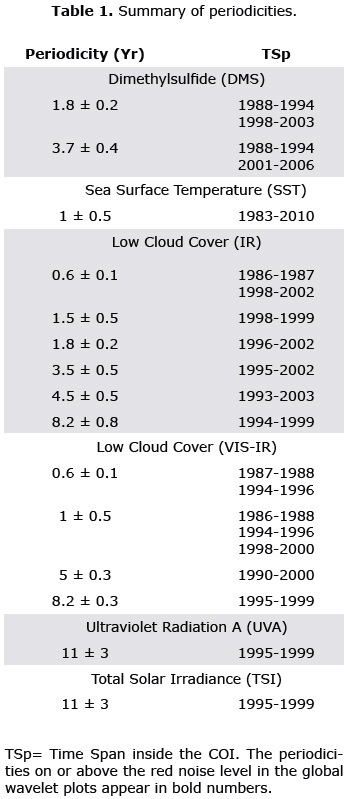
The results of the wavelet method are shown in Figure 1, a summary of the periodicities found for all the time series is shown in Table 1. The DMS global wavelet spectrum (Figure 1a) shows significant periodicities ~2 and 4 years. The SST global wavelet spectrum (Figure 1b) shows only one periodicity close to 1 year. The LCC-IR global wavelet spectrum (Figure 1c) presents significant peaks ~0.6, 1.5, 2 and 8 years, and the LCCVIS-IR global spectrum has significant periodicities ~0.6, 1, 5 and 8 years but taking into account the uncertainties these peaks coincide with the LCC-IR peaks. The UVA and TSI global wavelet spectrum (Figures 1e and 1f) show that the 11-years periodicity has the largest power, however its significance is low and partially outside the COI due to the short time interval.

 

The wavelet coherence spectra

The results of the wavelet coherence analysis appear in Figure 2 and present the coherence analysis between DMS vs SST, DMS vs LCC-IR, DMS vs LCCVIS-IR, DMS vs UVA and DMS vs TSI respectively. For each panel, the time series appears at the top, the wavelet coherence spectrum appears at the middle and the global wavelet coherence spectra is at the right. Table 2 summarizes the results; the strongest periodicities appear in bold number.

The Figure 2a shows that the DMS and SST time series have the most persistent and prominent coherence ~1 year and tends to be in phase, moreover, periodicities ~0.4, 2 and ~4 years, also notable in the wavelet coherence are mainly in phase, the wavelet coherence spectra analysis show an intermittent but sustained correlation between the analyzed series.

The coherences between DMS and LCC-IR and LCCVIS-IR appearing in Figures 2b and 2c do not show a definite phase. The Figure 2d shows that the DMS and UVA time series have the most persistent and prominent coherence ~0.5, 1 and 3 year and tend to be in anti-phase, the anticorrelation (anti-phase) is intermittent but sustained; while the peak ~8 years is in phase but outside the COI due to the time interval of the series.

The Figure 2e shows that the DMS and TSI time series have the most persistent and prominent coherence ~2 years and tends to be in anti-phase, moreover, persistent coherence at ~0.4 and 1 year is out of phase and ~8 years is in phase but outside the COI due to the time interval of the series.

The periodicities found are between ~0.4 and ~8 years. Peaks shorter than 1 year may be due to seasonal climatic phenomena. The ~2 years period can be associated with the Quasi-Biennial Oscillation (QBO) in the stratosphere (Holton et al., 1972; Dunkerton, 1997; Baldwin et al., 2001; Naujokat, 1986; Holton et al., 1980) and with the solar activity (Kane, 2005). The QBO dominates the variability of the equatorial stratosphere and is easily seen as downward propagating easterly and westerly wind regimes, with a variable period averaging approximately 28 months. The QBO is a tropical phenomenon; it affects the stratospheric flow from pole to pole by modulating the effects of extratropical waves. The QBO is present also in other stratospheric parameters not only tropical but also extra-tropical weather and other regions, as the mesosphere and troposphere. There is an established body of literature (Roy and Haigh, 2011; Labitzke, 2012; Weng, 2012), initiated by the pioneering work of Labitzke (1987), which has identified the influence of solar activity on the QBO.

In particular, it was found that by segregating the meteorological data by the QBO phase a clear signal of the 11-year solar cycle was revealed. More specifically, that the January-February temperature at 30 hPa over the North Pole tends to be warmer during the west phase of the QBO at high solar activity (HS/wQBO) and also during the east phase at low solar activity (LS/eQBO). Consistently, cold polar temperatures occur during LS/wQBO and HS/eQBO (Labitzke and van Loon, 1992). Other results suggest that solar variability, modulated by the phase of QBO, influences zonal mean temperatures at high latitudes in the lower stratosphere, in the mid-latitude troposphere and sea level pressure near the poles (Roy and Haigh, 2011).

The periodicities ~3 and 4 years could be related to the El Niño-Southern Oscillation (ENSO) (Nuzhdina, 2002; Njau, 2006) and to a sunspot periodicity (Polygiannakis et al., 2003).

The ENSO is the result of a cyclic warming and cooling of the surface ocean of the central and eastern Pacific, it occurs at irregular intervals between 2 and 7 years in conjunction with the Southern Oscillation, a massive seesawing of atmospheric pressure between the southeastern and the western tropical Pacific.

The ENSO leads to changes in ocean temperature that influence salinity changing environmental conditions for marine ecosystems. These changes affect fish populations, marine phytoplankton and chlorophyll. The direct influence of ENSO is reflected in the ocean, marine biota and climate. Recent work suggest an ENSO- like response to the 11-year solar cycle that includes a La Niña like pattern assigned to solar maximum conditions (Bal et al., 2011). The solar activity has obvious influence on some large scale climatic phenomena, such as ENSO. Kirov and Georgieva (2002) found that solar activity influenced both the intensity and occurrence frequency of the ENSO.

Mufti and Shah (2011) found a significant positive correlation between the SST anomalies and sunspot indices in both the 11-year and 22-year bands. Similar results showing correlation between solar activity and El Niño are also shown by Weng (2005). The influences of solar activity on the different natural processes are broad and extensive. However, large scale climatic phenomena, including ENSO, North Atlantic Oscillation (NAO), Atlantic Oscillation (AO), QBO) and Pacific Decadal Oscillation (PDO), present also periodicities that coincide with the solar activity cycles (Velasco and Mendoza, 2008), and also affect natural processes directly (Labat, 2010).

The periodicities ~5 years can be a harmonic of the 11-years solar cycle (Djurović and Páquet, 1996) and the periodicity ~8 years could be related to the 11-years sunspot cycle (taking into account the uncertainties). Summarizing, our results indicate a consistent correlation between DMS and SST and an anticorrelation between DMS-UVA. Between DMS-TSI we notice mainly an out of phase situation implying a nonlinear relationship. And the relation between DMS and LCCIR and LCCVIS-IR presents undefined phases indicating that the relation is also non-linear. The anticorrelation between UVA and DMS indicate a positive feedback, as discussed in other works (Larsen, 2005) or as implied by the findings of other papers (Mendoza and Velasco, 2009; Lockwood, 2005; Kristjánsson et al., 2002).

 

Conclusions

We studied the relationship between DMS and SST, LCC-IR, LCCVIS-IR, UVA and TSI using the Wavelet Method. We found dominant periodicities that coincide with those of large scale atmospheric phenomena or solar activity, for instance, the periodicities ~2 years can be associated to the Quasi-Biennial Oscillation (QBO) in the stratosphere as this atmospheric phenomenon is related to solar activity, those periodicities ~3 and ~4 years could be associated to the El Niño-Southern Oscillation (ENSO) as large scale climatic phenomena seem also influenced by solar activity, and the periodicities ~5 years can be associated a harmonic of the 11-year solar cycle. The results of the wavelet analysis show an intermittent but sustained correlation (phase) between DMS-SST and an anticorrelation (anti-phase) between DMS-UVA, these two cases indicate a linear relationships because the coherence of the series is high. The relations between DMS and TSI and LCC imply nonlinear relationships. The time-span of the series allow us to study only periodicities shorter than 11years, then we limit our analysis to the possibility that solar radiation influences the Earth climate in periods shorter than the 11-year solar cycle. Our results also suggest a positive feedback interaction between DMS and UVA solar radiation.

 

Bibliography

Andreae M.O., Crutzen P.J., 1997, Atmospheric aerosols: biogeochemical sources and role in atmospheric chemistry, Science 276, 1052–1058.         [ Links ]

Bal S., Schimanke S., Spangehl T., Cubasch U., 2011, On the robustness of the solar cycle signal in the Pacific region, Geophys. Res. Lett., 38, L14809.         [ Links ]

Baldwin M.P., Gray L.J., Dunkerton T.J., Hamilton K., Haynes P.H., Randel W.J., Holton J.R., Alexander M.J., Hirota I., Horinouchi T., Jones D.B., Kinnersley J.S., Marquardt C., Sato K., Takahashi M., 2001, The Quasi-Biennial Oscillation, Reviews of Geophysics, 39, 2, 179-229.         [ Links ]

Charlson R.J., Lovelock J.E., Andreae M.O., Warren S.G., 1987, Oceanic phytoplankton, atmospheric sulfur, cloud albedo and climate: a geophysiological feedback, Nature, 326, 655–661.         [ Links ]

Chen T., Rossow B.W., Zhang Y., 1999, Radiative effects of Cloud-Type variations, Journal of climate, 13.         [ Links ]

DeLand M.T., Cebula R.P., 2008, Creation of a composite solar ultraviolet irradiance data set. J. Geophys. Res. 113, A11103.         [ Links ]

Djurovic D., Páquet P., 1996, The common oscillations of solar activity, the geomagnetic field, and the earth's rotation, Solar Physics, 167, 427-439.         [ Links ]

Dunkerton T.J., 1997, The role of gravity waves in the quasi-biennial oscillation, J. Geophys. Res., 102, 26,053-26,076.         [ Links ]

Farge M., 1992, Wavelet transforms and their applications to turbulence, Annual Review of Fluid Mechanics 24, 395-457.         [ Links ]

Fröhlich C., 2009, Observational evidence of a long-term trend in total solar irradiance, Astron. Astrophys., 501, 27-30.         [ Links ]

Gallego D., Ribera P., Garcia-Herrera R., Hernandez E., Gimeno L., 2005, A new look for the Southern Hemisphere jet stream, Climate Dynamics, 24, 6, 607-621.         [ Links ]

Gilman D.L., Fugliste E.J., Mitchell J.R., 1963, On the power spectrum of Red Noise, Atmospheric Sciences 20, 182-184.         [ Links ]

Gray L.J., Beer J., Geller M., Haigh J.D., Lockwood M., Matthes K., Cubasch U., Fleitmann D., Harrison G., Hood L., Luterbacher J., Meehl G.A., Shindell D., Van Geel B., White W., 2010, Solar Influences on Climate, Reviews of Geophysics, 48, RG4001, 53 PP.         [ Links ]

Grinsted A., Moore J., Jevrejera S., 2004, Application of the cross wavelet transform and wavelet coherence to geophysical time series, Nonlinear Processes in Geophysics 11, 561-566.         [ Links ]

Gunson J.R., Spall S.A., Anderson T.R., Jones A., Totterdell I.J., Woodage M.J., 2006, Climate sensitivity to ocean dimethylsulphide emissions, Geophys. Res. Lett. 33, L07701.         [ Links ]

Häder D.P., Helbling E.W., Williamson C.E., Worrest R.C., 2011, Effects of UV radiation on aquatic ecosystems and interactions with climate change, Photochem. Photobiol.Sci., 242-260.         [ Links ]

Häder D.P., Kumar R.C., Smith R.C., Worrest R.C., 2003, Aquatic ecosystems: effects of solar ultraviolet radiation and interactions with other climatic change factors, Journal of the Royal Society of Chemistry, 39-50.         [ Links ]

Hardman-Mountford N., Hirata T., Richardson K., Aiken J., 2008, An objective methodology for the classification of ecological pattern into biomes and provinces for the pelagic ocean, Remote Sens. Environ., 112, 3341-3352.         [ Links ]

Hefu Y., Kirst G.O., 1997, Effects of UV radiation on DMS content and DMS formation of Phaeocystis Antartica, Polar Biol., 18, 402-409.         [ Links ]

Holton J.R., Lindzen R.S., 1972, An updated theory for the Quasi-Biennial cycle of the tropical stratosphere, Journal of the Atmospheric Sciences, 29, 1076-1080.         [ Links ]

Holton J.R., Tan H.C., 1980, The influence of the equatorial Quasi-Biennial Oscillation on the global atmospheric circulation at 50mb, Journal of Atmospheric Science., 37, 2200-2208.         [ Links ]

Kane R., 2005, Differences in the quasi-biennial oscillation and quasi-triennial oscillation characteristics of the solar, interplanetary, and terrestrial parameter, Journal of Geophysical Research, 110, 13.         [ Links ]

Kettle A.J., Andreae M.O., Amouroux D., et al., 1999, A global data base of sea surface Dimethylsulfide (DMS) measurements and a procedure to predict sea surface DMS as a function of latitude, longitude and month, Global Biogeochemical Cycles 13, 399-444.         [ Links ]

Fröhlich C., 2009, Observational evidence of a long-term trend in total solar irradiance, Astron. Astrophys., 501, 27-30.         [ Links ]

Kirov B., Georgieva K., 2002, Long-term variations and interrelations of ENSO, NAO and solar activity, Phys. Chem. Earth, 27, 441-448.         [ Links ]

Kniventon D.R., Todd M.C., Sciare J., Mihalopoulos N., 2003, Variability of atmospheric dimethylsulphide over the southern Indian Ocean due to changes in ultraviolet radiation, Global Biogeochem. Cycles, 17, 1096.         [ Links ]

Kristjánsson J.E., Staple A., Kristiansen J., Kaas E., 2002, A new look at possible connection between solar activity, clouds and climate, Geophys. Res. Lett., 29, 2107.         [ Links ]

Labat D., 2010, Cross wavelet analysis of annual continental freshwater discharge and selected climate indices, J. Hydrol., 385, 269–278.         [ Links ]

Labitzke K., 1987, Sunspots, the QBO and the stratospheric temperature in the north polar region, Geophys. Res. Lett., 14, 535-537.         [ Links ]

Labitzke K., van Loon H., 1992, On the association between the QBO and the extratropical stratosphere, J. Atmos. Terr. Phys., 54, 1453–1463.         [ Links ]

Labitzke K., Kunze M., 2012, Interactions between the stratosphere, the sun and the QBO during the northern summer, Journal of Atmospheric and Solar-Terrestrial Physics, 141, 75-76.         [ Links ]

Larsen S.H., 2005, Solar variability, dimethylsulphide, clouds and climate, Global Biogeochem. Cycles, 19, GB1014.         [ Links ]

Lean J.R., Lee G.J., Woods H., Hickey T.N., Puga J., 1997, Detection and parameterization of variations in solar mid- and near-ultraviolet radiation (200–400 nm), Geophys. Res. Lett. 102, 939-956.         [ Links ]

Lockwood M., 2005, Solar outputs, their variations and their effects on Earth, in The Sun, Solar Analogs and the Climate, Saas-Fee Advanced Course, 34, 109-306, Springer, the Netherlands.         [ Links ]

Longhurst A., Sathyendranath S., Platt T., Caverhill C., 1995, An estimate of global primary production in the ocean from satellite radiometer data, J. Plankton Res., 17, 1245-1271.         [ Links ]

Mendoza B., García-Acosta V., Velasco V., Jáuregui E., Díaz-Sandoval R., 2007, Frequency and duration of historical droughts from the 16th to the 19th centuries in the Mexican Maya lands, Yucatan Peninsula. Climatic Change.         [ Links ]

Mendoza B., Velasco V., 2009, High-Latitude Methane Sulphonic Acid Variability and Solar Activity. J. Atm. and Solar-Terr. Phys., 71, 33-40.         [ Links ]

Miller A.J., Alexander M.A., et al. 2003, Potential feedbacks between Pacific Ocean ecosystems and interdecadal climate variations, Bull. Am. Meteorol. Soc., 84, 617-633.         [ Links ]

Mufti S., Shah G.N., 2011, Solar-geomagnetic activity influence on Earth's climate, J. Atmos. Solar Terr. Phys., 73, 13, 1607-1615.         [ Links ]

Naujokat B., 1986, An update of the observed Quasi-Biennial Oscillation of stratospheric winds over the tropics, Journal of the Atmospheric Sciences, 43, 1873-1877.         [ Links ]

Njau E.C., 2006, Solar activity, El Niño-Southern oscillation and rainfall in India, Pakistan Journal of Meteorology, 3.         [ Links ]

Nuzhdina M.A., 2002, Connection between ENSO phenomena and solar and geomagnetic activity, Natural Hazards and Earth System Sciences, 83-89.         [ Links ]

Pidwirny M., 2006, Upper Air Winds and the Jet Streams, Fundamentals of Physical Geography, 2nd Edition.         [ Links ]

Polygiannakis J., Preka-Papadema P., Moussas X., 2003, On signal noise decomposition of time series using the continuous wavelet transform: application to sunspot index, Mon. Not. R. Astron. Soc., 343, 725–734.         [ Links ]

Ricchiazzi P., Yang S., Gautier C., Sowle D., 1998, SBDART: A Research and teaching software tool for plane-parallel radiative transfer in the Earth's atmosphere, Bull. Amer. Meteor. Soc. 79, 2101-2114.         [ Links ]

Roy I., Haigh D., 2011, The influence of solar variability and the quasi-biennial oscillation on sea level pressure, Atmos. Chem. Phys. Discuss., 10, 30452-30471.         [ Links ]

Rossow W.B., Schiffer R.A., 1999, Advances in understanding clouds from ISCCP, Bull. Am. Meteor. Soc. 80, 2261-2287.         [ Links ]

Sarmiento J.L., Gruber N., Brzezinski M.A., Dunne J.P., 2004, High-latitude controls of thermocline nutrients and low latitude biological productivity, Nature, 427, 6969, 56-60.         [ Links ]

Savitskiy G., Lessing, V., 1979, Tropospheric jet streams in the Antarctic, Polar Geography, 3, Iss. 3.         [ Links ]

Shaw G.E., Benner R.L., Cantrell W., Veazey D., 1998, The regulation of climate: A sulfate particle feedback loop involving deep convection-An editorial essay, Climate Change 39, 23–33.         [ Links ]

Simó R., 2001, Production of atmospheric sulfur by oceanic plankton: biogeochemical, ecological and evolutionary links, Trends in Ecology and Evolution, 16, 287–294.         [ Links ]

Simó R., Dachs J., 2002, Global ocean emission of dymethylsulfide predicted from biogeophysical data, Global Biogeochem. Cycles, 16.         [ Links ]

Simó R., Vallina S.M., 2007, Strong relationship between DMS and the solar radiation dose over the global surface ocean, Science, 315, 506-508.         [ Links ]

Slezak D., Herndl G.J., 2003, Effects of ultraviolet and visible radiation on the cellular concentration of dimethylsulfoniopropionate (DMSP) in Emilianiahuxleyi (strain L), Mar. Ecol. Prog. Ser. 246, 61-71.         [ Links ]

Toole D.A., Slezak D., Kiene R.P., Kieber D.J., 2006, Effects of solar radiation on dimethylsulfide cycling in the western Atlantic Ocean, Deep-Sea Res. I, 53, 136-153.         [ Links ]

Toole D.A., Siegel D.A., 2004, Light-driven cycling of Dimethylsulfide (DMS) in the Sargasso Sea: Closing the Loop, Geophys. Res. Lett., 31-9.         [ Links ]

Torrence C., Compo G.B., 1998, A practical guide to wavelet analysis, Amer. Meteor. Soc. 79, 61-78.         [ Links ]

Valdés-Galicia J., Velasco V., 2008. Variations of mid-term periodicities in solar activity physical phenomena, Advances in Space Research 41, 297-305.         [ Links ]

Vallina S.M., Simó R., Gassó S., DeBoyer-Montégut C.D., Jurado E., Dachs J., 2007, Analysis of a potential "solar radiation dose-dimethylsulfide-cloud condensation nuclei" link from globally mapped seasonal correlations, Global Biogeochem. Cycles, 21.         [ Links ]

Velasco V., Mendoza B., 2008, Assessing the relationship between solar activity and some large scale climatic phenomena, Advances in Space Research, 42, 866–878.         [ Links ]

Weng H., 2005, The influence of the 11 yr solar cycle on the interannual-centennial climate variability, J. Atmos. Solar Terr. Phys., 67, 793–805.         [ Links ]

Weng H., 2012, Impacts of multi-scale solar activity on climate. Part II: Dominant timescales in decadal-centennial climate variability, Advances in Atmospheric Sciences, 29, 887-908.         [ Links ]