Original paper

 

Characterization of ground motions using recurrence plots

 

Silvia R. García,¹* Miguel P. Romo¹ and Jesús Figueroa-Nazuno²

 

¹ Coordinación de Geotecnia, Instituto de Ingeniería, Universidad Nacional Autónoma de México. Ciudad Universitaria, Apartado Postal 70-472, México D.F., México. *Corresponding author: sgab@pumas.iingen.unam.mx

² Laboratorio de Computación Paralela y Distribuida Centro de Investigación en Computación, Instituto Politécnico Nacional, Av. Juan de Dios Bátiz, Apartado Postal 75-476, México, D.F., México.

 

Received: February 27, 2012
Accepted: January 10, 2013
Published on line: June 28, 2013

 

Resumen

Los modelos matemáticos tradicionales relacionados con el análisis de los terremotos son lineales y en algunos casos son incapaces de predecir determinados comportamientos, porque los datos que modelan pueden ser altamente no lineales y complejos. En este trabajo se describe la implementación de un método alternativo para el análisis sísmico en series de tiempo. La herramienta Mapas de Recurrencia (MR) permite el reconocimiento y el tratamiento de las aceleraciones medidas. Un Mapa de Recurrencia (MR) obtenido de datos sísmicos permite una interpretación más eficiente de los movimientos del suelo y la aplicación de esta explicación a la definición de estratigrafía y de las tendencias de respuesta. Los atributos no lineales obtenidos a partir del análisis de Mapas de Recurrencia se pueden utilizar como filtros para revelar patrones, o en combinación para predecir una propiedad sísmica. La caracterización automatizada de datos sísmicos, basada en los atributos sísmicos no lineales, podría rescribir las reglas de interpretación del fenómeno sísmico. El objetivo de este trabajo es establecer una metodología para la aplicación práctica de la dinámica no lineal en el reconocimiento de patrones sísmicos, un campo de la ingeniería desafiante y en constante evolución.

Palabras clave: mapas de recurrencia, series de tiempo sísmicas, caos análisis no lineal, movimientos fuertes de terreno, periodo fundamental del suelo, vibraciones en masas de suelo.

 

Abstract

The current analysis of earthquakes is typically based on linear mathematical models that may fail to describe and forecast particular behaviors, because in many cases the data complexity may induce a highly non linear behavior. In this paper the implementation of an alternative method for seismic time series analysis is presented. The RPs (Recurrence Plots) enables recognition and treatment of measured accelerations. An RP obtained from seismic data allows a more efficient interpretation of the ground motions and this explanation contributes to characterize materials and responses. The nonlinear attributes from RPs analysis can be used as filters to reveal patterns or be combined to predict a seismic property. Automated seismic data characterization, based on nonlinear seismic attributes, could rewrite the rules of earthquake phenomena interpretation. The objective of this work is to establish a new methodology for practical application of nonlinear dynamics in seismic pattern/attributes recognition, an evolving and challenging engineering field.

Key words: recurrence plots, seismic time series, nonlinear analysis chaos, strong ground motions, soil natural periods, soil vibrations.

 

Introduction

Data analysis often requires the drawing of meaningful conclusions about complicated systems using time-series data from a single sensor. The problem is rather complex because there usually exists simultaneously overabundance and lack of data: megabytes of time-series data about one parameter but no information regarding other important quantities. Data-mining techniques (Fayyad, 1996) provide some useful ways to deal successfully with the sheer volume of information that constitutes one part of this challenge. The second part is much harder. If the target system is highly complex say, a sudden release of strain/energy accumulated during extensive time intervals in the upper part of the Earth in the form of seismic waves radiated out in all directions from the source region through the Earth's interior and recorded at large distances by sensitive seismographs, but only a few of its important properties (e.g., surface acceleration) is sensor accessible, the data analysis procedure would appear to be fundamentally limited.

Figure 1 shows a simple example of the kind of problem that this work addresses: a mechanical spring/mass system and two time-series data sets gathered by sensors that measure the position and velocity of the mass. This system is linear: it responds in proportion to changes. Pulling the mass twice as far down, for instance, will elicit an oscillation that is twice as large, not one that is 2^1.5 as large or log2 times as large. A pendulum in contrast reacts according to a non linear relationship: if it is hanging straight down, a small change in its angle will have little effect, but if it is balanced at the inverted point, minor changes have significant effects in its response. This distinction is extremely important to science in general and for data analysis in particular. If the system under examination is linear, data analysis is comparatively straightforward and the tools are well developed. The data can be characterized by using statistics (mean, standard deviation, etc.), fit curves to them (functional approximation), and plot various kind of graphs to aid understanding of the behavior. If a more-detailed analysis is required, the system can be represented in an "input + transfer function → output" manner using any of a wide variety of time- or frequency-domain models. This kind of formalism admits a large collection of powerful reasoning techniques, such as superposition and the notion of transforming back and forth between the time and frequency domains.

Nonlinear systems pose an important question to intelligent data analysis. Not only they are ubiquitous in science and engineering, but their mathematics is also vastly harder and many standard time series analysis techniques simply do not apply to nonlinear problems. Real systems exhibit broad band behavior which makes that many traditional signal processing operations become useless. Non linear problems cannot be decomposed in the standard "input + transfer function → output" manner, nor can the noise be removed by simply low-pass filter data. The concept of a discrete set of spectral components does not make sense in many nonlinear problems, so using transforms to move between time and frequency domains does not work.

Another common complication in data analysis is observability: access to enough information to fully describe the system. The spring/mass system in Figure 1, for instance, has two state variables, the position and velocity of the mass, and both of them can be measured in order to know the state of the system. But for complex problems, the question is how to identify all of the internal state variables of the system and infer their values from the signals that can be observed. Geoseismic (geotechnical and seismological) procedures require accurate conclusions about reconstructed dynamics because fully observable systems are rare in geotechnical and earthquake engineering practice; as a rule, many often, most of a system's state variables either are physically inaccessible or cannot be measured with available sensors.

Based on the existing parameters, countless seismic attributes (measurements derived from seismic data) has been defined and introduced in seismic exploration (Sheriff, 1991; Brown, 1996; Chen and Sidney, 1997; and Eastwood, 2002). Many of these attributes play exceptionally an important role in interpreting and analyzing data (Chopra and Marfurt, 2005) however, many questions remain unanswered about the effectiveness and practicality of using these conventional (linear and stationary) techniques on earthquake phenomena. In this work a more useful time-series analysis procedure is presented.

The aim of this investigation is to apply the concepts of chaos theory to global characterization of the soil deposits through the structures of the two-dimensional images, Recurrence Plots RPs (Eckmann et al. 1986) constructed from acceleration time series. The RPs-methodology proposed here, general and practical, uses the structures of the accelerograms for a "topological" interpretation of the data. Through visualization and quantitative assessment of these configurations, the manifestations of soil (heterogeneous materials vibrating) can be described. We demonstrate the potential capability of RPs using events recorded in Mexico City (rock and soft-soil deposits) during minor and extreme seismic events.

 

Studying Complex Systems

When a researcher must deal with large data sets, the expert should adopt or develop specific analyses for classification, visualization, understanding and manipulation of the time series in order to understand more about the underlying system and to determine the direction of future research. Traditional methods of time series analysis come from the well-established field of digital signal processing (Abarbanel, 1996). One of the most familiar and widely used tools is the Fourier transform. Indeed, many traditional methods of analysis, visualization, or processing uses the Fourier transform in order to change a set of linear differential equations into an algebraic problem where powerful methods of matrix manipulation may be used. However, these methods are designed to deal with a restricted subclass of possible data. The data is often assumed to be stationary -that means, independent of time. It is also assumed that the dynamics are fairly simple, both low-dimensional and linear. Compound this with the additional assumptions of low noise and a non broad-band power spectrum, then it can be seen that a very limited class of data is implied. With experimental nonlinear data, as the ground accelerations measured during an earthquake, this traditional signal processing methods may fail because the system dynamics are, at best, complicated, and at worst, extremely noisy.

An example to illustrate this point is depicted in Figure 2. Fourier transform is applied to data (acceleration time series) from a soft soils deposit (site named as SCT) when is affected by seismic load (four events). If natural period (fundamental frequency), stratigraphy and topographical/geometrical conditions are held constant (same recording station) then the differences between the response representations must be related with the fault mechanism, magnitude, distance (source-site) and directivity. See the spectra of two events from the same seismogenic zone (epicenters circled together that means for practical purposes, same fault, distance and radiation pattern) shown in Figure 2a. The frequency content is very similar and the obvious difference between these representations is the intensity level. What additional variables (if any) are needed to explain the remarkable distance between shaking energies? In Figure 2b two responses due to seismic events generated by different fault mechanisms, thus having dissimilar directivities and distances, are shown. As can be seen, these Fourier representations have very similar frequency-intensity distribution and it can be assumed that they might produce the same structural or architectural damage. Since they result from very different seismic activity, which conditions or parameters must be defined in order to justify the strong similitude between these responses? In these cases, the transformation to the frequency domain is restrictive and many important geological and seismic aspects could be ignored or misinterpreted.

What is needed is an alternative and reliable recording-based approach to explore, to characterize and to quantify earthquake-induced effects. Analysis from a nonlinear dynamics perspective may yield more fruitful results; still, this is not a straightforward task. Calculation of empirical global nonlinear quantities, such as Lyapunov exponents and fractal dimension, from time series data is known to often yield erroneous results (Ding et al., 1993; Parlitz, 1992). The literature is replete with examples of poor or erroneous calculations and it has been shown that some popular methods may produce circumspect results (Eckmann and Ruelle, 1992; Vastano and Kostelich, 1986). Limited data set size, noise, nonstationarity and intricate dynamics are presented as additional complications. The concerns about the data are compounded by concerns about analysis. It is expected that the following consistent synthesis of the RP-analysis will enable researchers to perform studies more efficiently and more confidently. Thus it is encouraged that first at all, the user familiarizes him with the background and the methodology before attempting any analysis. To make the paper self-contained, some key concepts of Chaos Theory and Recurrence Plots are presented in the following paragraphs.

Chaos Attractor

State Space Description

The state of a system is defined as the value of the smallest vector such that at time t₀ it completely determines the system behavior for any time t ≥ t₀ (Cao, 1997). The components of the state vector are called state variables. The evolution of a system can be visualized as a path in state space. Since a dynamical system must contain memory elements, integrators can be used to describe the state space representation. The evolution of the state space can therefore be described with the following equations:

where and are the system input and output respectively. This set of differential equations completely describes the system. The collection of all possible states is called the phase space. Thus, the phase space is a subset of the state space.

Equilibrium Points, Periodic Solutions, Quasiperiodic Solutions and Chaos.

As time goes to infinity, the asymptotic behavior of a system that is not purely noise-driven can be categorized as being one of four general types: equilibrium points, periodic solutions, quasiperiodic solutions, or chaos (Horai et al., 2002).

An equilibrium point can be either stable or unstable. Stable equilibrium points are called sinks, and unstable points are called sources. A sink causes that near trajectories move towards the self-sink with an increase in time, and this is an example of an attractor. When a trajectory precisely returns to itself, the system has a periodic solution with a fixed period T. The value of T is the time needed to reach the same point in state space again. A limit cycle is an example of an attractor that has a periodic solution. The period of a quasiperiodic system is not fixed, i.e. the phase space is formed by the sum of periodic solutions that have periods whose ratio is irrational.

Lorenz (Lorenz, 1963) discovered the first example of a chaotic attractor while searching for the solution of a weather prediction model. Qualitatively speaking, a chaotic attractor is an attractor that is not of the previous three types. A system of this type is very dependent on initial conditions, i.e. two points in state space that are separated by a small distance will diverge exponentially as the system evolves. Thus, the term "chaotic" describes a dynamical property of a system.

Modeling the Attractor

Having established that a system contains a chaotic attractor, the process can be modeled by reconstructing the state space. Two methods are available: the method of delays and principal component analysis. We will not give a detailed description of principal component analysis because in this investigation the method of delays is used. Thus, we refer the reader interested on the former method to Broomhead and King (1986).

Mutual Information. Frasier and Swinney (Fraser and Swenney, 1986) proposed mutual information method to obtain an estimate for delay time, τ (March et al., 2005). Mutual information provides a general measure for the dependence of two variables, thus, the value of τ for which the mutual information goes to zero is preferred. Additional arguments for choosing the first zero can be found in (Saussol and Wu, 2003).

Mutual information is a measure found in the field of Information Theory. Let S be a communication system with s₁,s₂,...,s_n a set of possible messages with associated probabilities P_s (s₁ ), P_s (s₂ ),...,P_s (s_n).

The entropy H of the system is the average amount of information gained from measuring s and it is defined as

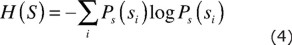
For a logarithmic base of two, H is measured in bits. Mutual information measures the dependency of x(t + T). Let [s,q]=[x(t),x(t+T)], and consider a coupled system (S,Q). Then, for sent message s and corresponding measurement s_i,

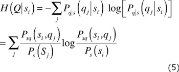
where is the probability that a measurement of q will result in q_j, subject to the condition that the measured value of s is s_i. Next we take the average uncertainty of over s_i,

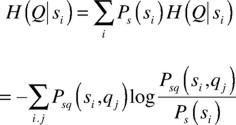
= H(S,Q) − H(S) (6)

with

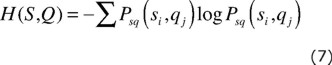
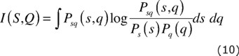
The reduction of the uncertainty of q by measuring s is called the mutual information I(S,Q) which can be expressed as

I(Q,S) = H(Q) − H(Q|S) (8)

= H(Q) + H(S) − H(S,Q) = I(S,Q) (9)

where H(Q) is the uncertainty of q in isolation. If both S and Q are continuous, then

If s and q are different only as a result of noise, then I(S,Q) gives the relative accuracy of the measurements. Thus, it specifies how much information the measurement of x_i provides about x_i+1. The mean and variance of the mutual information estimation can be calculated (Takens, 1981). Although mutual information guarantees decorrelation between x_k and x_k+t, and between x_k+t and x_k+2t, it does not necessary follow that x_k and x_k+2t are also uncorrelated (Afraimovich et al., 2003).

False Nearest Neighborhoods. Mutual information gives an estimate for τ_s, but does not determine the embedding dimension d. The Takens' Theorem (Takens, 1981) states that an m-dimensional attractor will be completely unfolded with no self-crossings if the embedding dimension is chosen larger than 2m. In this work, the method of false nearest neighbors is used for finding a good value for d (Afraimovich, 1997).

The method is based on the idea that two points close to each other (called neighbors) in dimension d, may in fact not be close at all in dimension d+1. This can happen when the lower dimensional system is simply a projection of a higher dimensional system, and it is unable to completely describe the system. Thus, the algorithm searches for "false nearest neighbors" by identifying candidate neighbors, increasing the dimension, and then inspecting the candidate neighbors for false ones. When no false neighbors can be identified, it is assumed that the attractor is completely unfolded and d, at this point, taken as the embedding dimension.

Recurrence Analysis

In our daily life we make predictions that are not based on the evaluation of long and complicated sets of mathematical equations, but rather on two crucial facts: i) similar situations often evolve in a similar way; ii) some situations occur over and over again. The first fact is linked to certain determinism in many real world systems. Chaos theory has taught us that some systems - although deterministic- are very sensitive to fluctuations and even the smallest perturbations of the initial conditions can make a precise prediction on long time scales impossible. The second fact is fundamental to many systems and it is probably one of the reasons why life has developed memory. Experience allows remembering similar situations, making predictions and, hence, helps to survive. But remembering similar situations is only helpful if a system returns or recurs to former states. Such a recurrence is a fundamental characteristic of many dynamical systems and it can indeed be used to study their properties.

The set of nonlinear dynamic techniques, called Nonlinear Time Series Analysis (Kantz and Schreiber, 1997), can be classified into metric, dynamical, and topological tools. The metric approach depends on the computation of distances on the system's attractor. The dynamical approach deals with computing the way nearby orbits diverge by means of estimating Lyapunov exponents. Topological methods are characterized by the study of the organization of the strange attractor, and they include close returns plots and Recurrence Plots RPs (Eckmann et al., 1986).

Recurrence Plots

RPs are intricate and visually appealing. They are also useful for finding hidden correlations in highly complicated data. In this work the RP-analysis is extended, formalized, and systematized in a meaningful way that is based both in theory and experiments and that targets both quantitative and qualitative properties for its geotechnical and seismological application.

In this section, we briefly outline some of the basic features of RPs and describe how an RP of an experimental data set can be generated. The standard first step in this procedure is to reconstruct the dynamics by embedding the one-dimensional time series in a d_E-dimensional reconstruction space using the method of delay coordinates. Given a system whose topological dimension is d, the sampling of a single state variable is equivalent to projecting the d-dimensional phase-space dynamics down onto one axis.

Loosely speaking, embedding is akin to "unfolding" those dynamics, albeit on different axes (Packard et al, 1980; Takens, 1981). Given a trajectory in the embedded space, finally, an RP is constructed by computing the distance between every pair of points (y_i,y_j) using an appropriate norm and then shading each pixel (i,j) according to that distance. The process of constructing a correct embedding is the subject of a large body of literature and numerous heuristic algorithms and arguments. Abarbanel (1995) gives a good summary of this extremely active field.

a) Delay Coordinate Embedding. To reconstruct the dynamics, we begin with experimental data consisting of a time series:

{x1,x2,...,xN} (11)

Delay-coordinate reconstruction of the unobserved and possibly multi-dimensional phase space dynamics from this single observable x is governed by two parameters, embedding dimension d_E and time delay τ. The resultant trajectory in is:

{y₁, y₂, ..., y_m} (12)

where m=N-(d_E-1)τ and

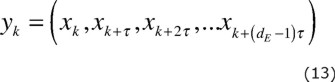
for k=1,2,..., m. Note that using d_E=1 merely returns the original time series; one dimensional embedding is equivalent to not embedding at all. Proper choice of d_E and τ is critical to this type of phase-space reconstruction and must therefore be done wisely; only "correct" values of these two parameters yield embeddings that are guaranteed by the Takens Theorem (Takens, 1981; Packard et al., 1980; Sauer et al., 1991) to be topologically equivalent to the original (unobserved) phase-space dynamics.

Assuming that the delay-coordinate embedding has been correctly carried out, it is natural to assume that the RP of a reconstructed trajectory bears great similarity to an RP of the true dynamics. Furthermore, we expect any properties of the reconstructed trajectory inferred from this RP to be true of the underlying system as well. This is, in fact, the rationale behind the standard procedure of embedding the data before constructing a RP.

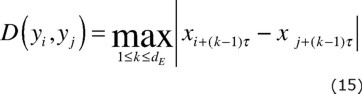
B) Constructing the Recurrence Plot. RPs are based upon the mutual distances between points on a trajectory, so the first step in their construction is to choose a norm D. In this work the maximum norm is used, although in one dimension the maximum norm is, of course, equivalent to the Euclidean p-norm. We chose the maximum norm for two reasons: for ease of implementation and because the maximum distance arising in the recurrence calculations (the difference between the largest and smallest measurements in the time series) is independent of embedding dimension d_E for this particular norm. This means that we can make direct comparisons between RPs generated using different values of d_E without first having to re-scale the plots. Next, we define the recurrence matrix A as follows:

A(i,j) = D(y_i,y_j), 1 ≤ i,j ≤ m (14)

follows

The time series spans both ordinate and abscissa and each point (i,j) on the plane is shaded according to the distance between the two corresponding trajectory points y_i and y_j (Figure 3). The pixel lying at (i,j) is color-coded according to the distance. For instance, if the 117th point on the trajectory is 14 distance units away from the 9435th point, the pixel lying at (117, 9435) on the RP will be shaded with the color that corresponds to a spacing of 14.

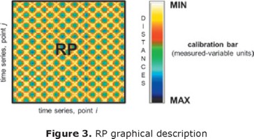
Figure 4 shows RPs generated from very different data sets: from a time series derived by sampling the function sine t until a noise series. The colors on these plots range from white-yellow for very small spacing to dark blue for large inter-point distances (see calibration bar in Figure 3). With this in mind, the sine-wave RP is relatively easy to understand; each of the "blocks" of color simply represents half a period of the signal. The lower RPs in the Figure 4 (see the ECG, Lorenz and Rössler RPs, for example), generated from chaotic data sets, are far more complicated, although they too have block-like structures resembling what might be expected from a periodic signal. These signals, though, are not periodic, so the repeated structural elements in the plot request a deeper explanation. The recurrent inter-point distances (repeated colors) are not straightforwardly related with the signals but it seems that some kind of determinism is presented in the behaviors. The RPs could be categorized following the knowledge about the systems that generated the signal and the particular array of the repeated structures. Alternatively, recurrence points for the white noise (at the bottom of Figure 4) are simply distributed in a homogeneous random pattern, signifying that the variable lacks of deterministic structures.

C) Structures in RPs. As already mentioned, the initial purpose of RPs was to visualize trajectories in phase space, which is especially advantageous in the case of high dimensional systems. RPs yield important insights into the time evolution of these trajectories, because typical patterns in RPs are linked to a specific behavior of the system. Following the phase space characteristics, the path in the correlation dimension curve and the large scale patterns in RPs, designated as typology, the RPs structures can be classified as homogeneous, periodic, drift and disrupted ones (Marwan, 2003):

• Homogeneous RPs are typical of systems in which the relaxation times are short in comparison with the time spanned by the RP. An example of such an RP is that of a stationary random time series. See the uniformly distributed white noise example shown in Figure 4.

• Periodic and quasi-periodic systems have RPs with diagonal oriented, periodic or quasi-periodic recurrent structures (diagonal lines, checkerboard structures). Figure 4 shows the RP of the sine signal, example of a periodic system. Irrational frequency ratios cause more complex quasi-periodic recurrent structures (see the ECG, Lorenz, Rössler and sun spots examples); however, even for oscillating systems whose oscillations are not easily recognizable, RPs can be very useful.

• A drift is caused by systems with slowly varying parameters, i.e. non-stationary systems. The RP pales away from the line of identity, LOI (the main diagonal line in a RP, Ri,j=1).

• Abrupt changes in the dynamics as well as extreme events cause white areas or bands in the RP, for example the Brownian motion (Figure 4). RPs allow finding and assessing extreme and rare events easily by using the frequency of their recurrences.

A closer inspection of the RPs reveals also the texture or small-scale structures (Eckmann et al., 1987), which can be typically classified in single dots, diagonal lines as well as vertical and horizontal lines (the combination of vertical and horizontal lines obviously forms rectangular clusters of recurrence points); in addition, even bowed lines may occur (Marwan, 2003; Eckmann et al., 1987):

• Single, isolated recurrence points can occur if states are rare, if they persist only for a very short time, or fluctuate strongly.

• A diagonal line (where l is the length of the diagonal line) occurs when a segment of the trajectory runs almost in parallel to another segment for l time units:

• A vertical (horizontal) line (with v the length of the vertical line) marks a time interval in which a state does not change or changes very slowly:

The state is trapped for some time. This is a typical behavior of laminar states (intermittency) (Marwan et al., 2002).

• Bowed lines are lines with a non-constant slope. The shape of a bowed line depends on the local time relationship between the corresponding close trajectory segments.

RPs of paradigmatic systems provide an instructive introduction into characteristic typology and texture but the visual interpretation of RPs requires some experience. To summarize the explanations about typology and texture, we present a list of features and their corresponding interpretation in Table 1.

 

RPs of Seismic Recordings

A set of acceleration time series recorded in the soft soils of the Mexican metropolis are used to study its chaotic nature. We first define the soil systems and then we classify the behavior and propose a nonlinear label.

Data base

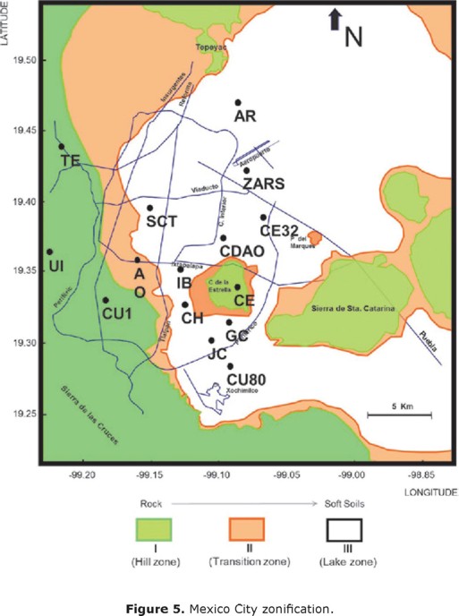
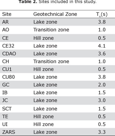
The recorded responses on the surface of 11 soft soils (clays) and 4 stiff deposits within the urban area of Mexico City conform the signals used in this study. These sites are located on the lacustrine basin where soils were deposited by air or water transportation (very soft clay formations with large amounts of microorganisms interbedded by thin seams of silty sand), some others are product of volcanic effusions that took place within the last one million years (fly ash and volcanic glass) and there are stations on a third type of soils that are considered firm or materials rock-like. Based on this material characterization and the historical seismic behavior, the Mexico valley has the geotechnical microzonation (Figure 5). This map is taken as a means of gaining broad insight into the surface motion of a particular site. The elastic natural periods T_n (key parameter in ground motions categorization) of the sites included in the database vary from T_n=1 s to T_n=4.2 s (Table 2).

The 9 events selected (Table 3), having at least 100 s and high signal-to-noise ratios, are representative of the tectonic regions (different source mechanism) that affects the valley. The set is denser in events from the subduction of the Cocos Plate into the Continental Plate because they are associated to the most damaging shocks.

Regular and chaotic ground motions

Information accumulated over the last four decades has firmly established that the singular geotechnical environment that prevails in Mexico City is the one most important factor to be accounted for in explaining the huge amplification of seismic movements. Also, observational evidence has made it clear that seismic movements within the Basin of Mexico can differ considerably from one site to the other (Romo and Seed, 1986). The statutory regulations have tried to take into account these facts but still there are dangerous doubts about the outcome patterns. The purpose of the following analysis is to illustrate an alternative way in which the oscillations can be described and to provide a qualitative understanding of the complex system responses.

RPs-Typology (large scale)

Examples of RPs obtained from accelerograms recorded during the earthquakes listed in Table 2, are shown in Figure 6. One intriguing and puzzling characteristic of the RPs is the structural similitude that they exhibit with different seismic and site conditions. Evaluating RPs constructed from accelerograms recorded during the same event on different site conditions (Figure 7), one question is obligated: do soft soils and rocks, when are excited by the same seismic force, have alike movements? On the other hand, keeping constant the soil properties (dividing the database in a subset of soft soils and a subset of rock deposits) and varying the seismic inputs (events), the RPs structures are exceptionally comparable (Figure 8) and the query is evident: do earthquake mechanism, distance (from epicenter to the site) and transmission pattern have significant impact on the way the materials vibrate?

Answering these questions using the large scale is a difficult task and requires the use of restricting assumptions in order to explain the behaviors and response trends. It is important to point out that the conventional time series analysis tools works on this scale.

Through a deep inspection of the RPs and using nonlinear concepts we can say that the ground structures (soft and stiff, homogeneous and heterogeneous deposits) when are affected by seismic forces, in a macro scale, evolve in a similar way. The time evolution of the ground accelerations exposes well defined white areas and cold bands (green/blue strips), hallmark in nonstationary systems. The combination of vertical and horizontal strips forms rectangular clusters where the maximum accelerations are located. Because of the abrupt changes between the beginning, the intense and the final part of the movements, a ground motion can be defined as an event that contain extreme sub-events (maximum accelerations) where the ground conditions are anomalous for some seconds to then vanish until the movement finishes. The number of clusters that appears in the RPs is the recurrence of the sub-events. The study of vertical RP structures makes the identification of trapping time (seconds that soil and rocks are being truly perturbed) possible.

To better understand the complexity of the ground motions, compare the RPs calculated from seismic time series with those from a pendulum's oscillation and damped vibration (low drive frequencies) depicted in Figure 9a. The ground response is very far from the deterministic behavior of this apparently simple device. See the RP in Figure 9b, the drive frequency is raised and the attractor undergoes a series of bifurcations (the pendulum is oscillating in a chaotic manner) but even in this regime the pendulum's RP manifests as seemingly structured with almost-periodic patterns. None of the RPs of accelerograms can be related with the patterns of the pendulum's attractors. The underlying process in seismic ground motions seems much more complex and it cannot be directly labeled as "deterministic", "chaotic" or "random".

The RPs-vertical structures displayed by the layered natural materials should be related with intermittence. In dynamical systems the intermittence is the alteration of phases of seemingly periodic systems. The apparent periodic phases of the ground behavior are not quite, but only nearly periodic. Thus, rather than a truly-periodic series of values, the data are apparently periodic but where the chaotic nature of the system becomes apparent after certain ground acceleration is reached. It is very important to point out that intermittence is more patent during large earthquakes, and a probably reason, which looks a paradox, is that the energy released from the source is not permanently continuous on time, there are relax intervals in between without important seismic wave arrivals from the source. Therefore the intermittence in accelerograms could be considered as a random sequence of episodes of seismic wave arrivals and episodes of free soil vibrations.

In a modeling scenario where the system was composed of many kilometers of crust (the outermost layer of the earth) from the source of seismic activity to the station where the measurement instrument registers the acceleration of a point on the ground surface (Figure 10), soils and rocks can be classified as nonlinear devices because they become activated when their reaction potential crosses a certain threshold. The activity of large formations of geological materials (soils and rocks) is macroscopically measurable in the accelerogram which results from a spatial integration of many reaction potentials (the environment interacting) but what is needed in the earthquake engineering is a description of the particular nonlinear devices (soil and rock deposits) through this macro manifestation, and this is the main advantage of RPs over the time-series analysis tools.

RPs-Texture (small scale)

Delay-coordinate embedding produces clean, easily analyzable pictures of the ground dynamics and the results suggest that the dynamical behavior of the soils/rocks is very high-dimensional (Table 4). This implies that the system is probably influenced by variables that can be hardly identified or that are beyond the limits of our current understanding (Strogatz, 2000). However, a proper definition of initial conditions permits characterizing the system evolutions and extracting meaningful (for engineering purposes) conclusions about the behavior of this complex natural structure.

Zooming into the RPs, the soil response can be studied from the clear and suggestive signatures in the clusters. The width of the vertical band indicates the time in which the intense state does not change or changes very slowly. The strong ground accelerations are trapped for some seconds (the cluster base) and because this extreme situation is not an isolated point (rare) the possibility that this alteration had been produced by noise is eliminated. In this intense time, periodic, chaotic or random patterns can be recognized and the parameters range over which the system is stable and where the trajectories are divergent could be identified.

Harmonics in soft soils oscillations. Observe the Figure 11. These clusters in the third column were obtained from accelerograms registered in soft soils deposits. These examples show diagonal oriented recurrent structures that can be related with the vibration of one degree of freedom 1D oscillator. Due to space restrictions only some examples are showed, but they are representative of the structures displayed for the whole soft-soils set.

Assuming that during intermittence soft soils behave as a 1D oscillator, the period of soil vibration during the semi-sinusoidal oscillation (in this investigation called T_ss) can be obtained from the distance between diagonals (Figure 12). For a same site, no important degradation is observed in T_ss, even when the records came from different intensity, frequency and duration input conditions. Beyond the scope of this work is the discussion about the impact of the differences between T_ss and T_n in the aseismic design, but no doubt exists that the T_ssvalues are more authentic than those obtained from spectral analyses and many important conclusions about nonlinearity and site effects must be re-evaluated using these findings.

Chaotic vibrations in stiff soils structures. The clusters in the first column of Figure 11 are far more complicated. The checkboard structures and the upward diagonal lines result from strings of vector patterns repeating themselves multiple times down the dynamics. This type of recurrent structure indicates that the dynamics is visiting the same region of an attractor at different times; therefore, the presence of diagonal lines indicates that deterministic rules are present in the dynamics. The set of lines parallel to the main diagonal is the signature of determinism, however, it is not so clear as in soft-soils (e.g., the size of the lines being relatively short among a field of scattered recurrent points), i.e., the RPs contain subtle patterns not easily ascertained by visual inspection.

Although the blocklike structures resembling to what might be expected from a periodic signal, the rock-like materials exhibit a complex recurrent behavior with irregular cyclicities that qualifies them as dynamical systems and their behavior as typical for nonlinear or chaotic systems. This means that the deposits in Hill zone are highly sensitive to initial conditions, e.g. small differences in directivity, fault mechanism or distance, yield widely diverging outcomes.

As in many natural systems, the geological materials constitute systems that can be called deterministic, meaning that their future behavior is fully determined by their initial conditions, with no random elements involved. The deterministic nature of rock (stiff materials) systems does not make them predictable. The rock-like deposits behavior can be described as deterministic chaos, or simply chaos.

Random signature in Transition zone. The clusters from sites, whose stratigraphy is erratic or not clearly defined, are distributed in a homogeneous random pattern, signifying that the random variable (accelerations) lacks of deterministic structures (see second column in Figure 11).

It seems that the location of the seismic source has not a strong influence on the characteristic of the RPs-clusters. From these observations we can conclude that seismic soil response is controlled by the dynamics of the fault that governs the time episodes of energy release, but the magnitude, the epicentral distance and the focal depth are not parameters that can fully categorize the random behaviors and Transition topologies in the RPs.

 

Conclusions

Based on the findings of this study, recorded accelerograms on soils and rocks should be considered as a sequence of episodes of seismic wave arrivals alternated with free soil vibrations episodes, behavior related with intermittence.

If we associate the clusters size with the concept of effective acceleration, the RPs can help to determine which level of acceleration is most closely related to structural response and to damage potential of an earthquake and which is its duration. The different durations are consequence, following with the assumption of intermittence, of the arrival of seismic waves at the end of the earthquake that excite soil/rock layers and which are attenuated (or amplified) depending of the periods and corresponding damping materials. It has been noticed, from the analyzed cases (different fault mechanisms, epicentral distances and magnitudes), that there are no significant differences between soil and rock time evolutions (macroscale). The study of the alteration of phases in RPs drives to the conclusion that soils and rocks deposits responses can be characterized only in the intense part of the time series. Soft soils deposits progress from quasi-periodic to periodic oscillations as the amplitude of the seismic responses exceeds certain acceleration thresholds. RPs of stiff materials, in general, display more complicated structures but they resemble chaotic movements for the universe of initial conditions analyzed. Despite being chaotic, the trajecto are actually quite organized, contrary to the RPs from erratic stratigraphies (Transition zone) whose are very close to being completely random.

The inconsistency between soil amplification theories and accelerographic measurements for large earthquakes could be re-interpreted through Chaos theory: Geological materials are systems that evolve in a similar way, so the amplification ratios should not be studied in the macro scale (even in the frequency domain). The deposits studied can be linked to certain determinism but they are very sensitive to initial conditions. The slightest change in initial conditions (stiffness material and intensity of the seismic waves arrivals, between the most important) or noise may cause the system to enter a very different trajectory.

This investigation permits to conclude that due to the inherent nonlinearities, the linear analysis techniques either fail or become meaningless to describe seismic responses and the spectral relations derived from these preprocessing techniques do not produce meaningful results.

Even if nowadays the consideration of non-linear seismic attributes is not necessary, it is undeniable that it will be needed in the future.

The future will see more multidimensional attributes with geotechnical, geological and seismological significance and a greater reliance on multi-attribute analysis. These trends are leading to automatic pattern recognition techniques for geoseismic analysis, able to rapidly characterize large volumes of data, or retrieve subtle details hidden in the data. Our aim is to propose a robust qualitative/quantitative method capable to identify and to characterize the seismic time series to be exploited in analysis and design procedures. Like search engines help you locate information on the worldwide web, the nonlinear tools built in your data viewer would locate features in your seismic records, as a "seismic search engine".

 

Bibliography

Abarbanel H.D., 1995, Analysis of Observed Chaotic Data. 1st ed., Springer-Verlag, New York.         [ Links ]

Afraimovich V., Chazottes J.R., Saussol B., 2003, Pointwise dimensions for Poincaré recurrences associated with maps and special flows, Discrete Conti. Dynam. Syst. A 9 (2) 263–280.         [ Links ]

Afraimovich V., 1997, Pesin's dimension for Poincaré recurrences, Chaos 7 (1) 12–20.         [ Links ]

Broomhead D.S. and King G.P., 1986, On the Qualitative Analysis of Experimental Dynamical Systems in 'Nonlinear Phenomena and Chaos' ed. S. Sarkar, Adam Hilger: Bristol 113 – 144        [ Links ]

Brown A. R., 1996, Seismic attributes and their classification, The Leading Edge, 15, 1090.         [ Links ]

Cao L., 1997, Practical method for determining the minimum embedding dimension of a scalar time series, Physica D, 110, 1–2, 43–50.         [ Links ]

Chen Q., Sidney S., 1997, Seismic attribute technology for reservoir forecasting and monitoring, The Leading Edge, 16, 5, 447-448.         [ Links ]

Chopra S., Marfurt K. J., 2005, Seismic attributes: A historical perspective, Geophysics, 70, 5, 3SO–28SO.         [ Links ]

Ding M., Grebogi C., Ott E., Sauer T., Yorke J. A., 1993, Plateau onset for correlation dimension: When does it occur?, Phys. Rev. Lett. 70, 3872–3875.         [ Links ]

Eastwood J., 2002, The attribute explosion, The Leading Edge, 21, 994.         [ Links ]

Eckmann J.P., Kamphorst S.O., Ruelle D., 1987, Recurrence plots of dynamical systems, Europhys. Lett. 5, 973–977.         [ Links ]

Eckmann J.P., Oliffson Kamphorst S., Ruelle D., and Ciliberto S., 1986, Lyapunov exponents from a time series, Phys. Rev. A 34, 4971.         [ Links ]

Eckmann J.P., Ruelle D., 1992, Fundamental limitations for estimating dimensions and Lyapunov exponents in dynamical systems, Physica D, 56, 185-187.         [ Links ]

Fraser A. M. and Swinney H. L., 1986, Independent coordinates for strange attractors from mutual information, Phys. Rev. A33 1134-1140.         [ Links ]

Fayyad U., Piatetsky-Shapiro G., Smyth P., Uthurusamy R., 1996, Advances in Knowledge Discovery and Data Mining, 1st ed., MIT Press.         [ Links ]

Horai S., Yamada T., Aihara K., 2002, Determinism analysis with isodirectional recurrence plots, IEEE Trans. Inst. Electric. Eng. Jpn. C 122 (1) 141–147.         [ Links ]

Kantz H., Schreiber T., 1997, Nonlinear Time Series Analysis, Cambridge University Press, Cambridge.         [ Links ]

Lorenz E.N., 1963, Deterministic nonperiodic flow, J. Atmos. Sci. 20, 130–141.         [ Links ]

March T.K., Chapman S.C., Dendy R.O., 2005, Recurrence plot statistics and the effect of embedding, Physica D 200,1–2, 171–184.         [ Links ]

Marwan N., 2003, Encounters with neighbours—current developments of concepts based on recurrence plots and their applications, Ph.D. Thesis, University of Potsdam.         [ Links ]

Marwan N., M.H. Trauth, M. Vuille, J. Kurths, 2003, Comparing modern and Pleistocene ENSO-like influences in NW Argentina using nonlinear time series analysis methods, Clim. Dynam. 21 (3–4) 317–326.         [ Links ]

Marwan N., Wessel N., Meyerfeldt U., Schirdewan A., Kurths J., 2002, Recurrence plot based measures of complexity and its application to heart rate variability data, Phys. Rev. E 66 (2).         [ Links ]

Packard N.H., Crutchfield J.P., Farmer J.D., Shaw R.S., 1980, Geometry from a Time Series, Phys. Rev. Lett, 45- 9, 712-716.         [ Links ]

Parlitz U., 1992, Identification of true and spurious Lyapunov exponents from time series Int. J. Bifurcat. Chaos, 2, 155–165.         [ Links ]

Sauer T., Yorke J.A., Casdagli M., 1991, Embedology, J. Stat. Phys. 65(3/4), 579-616.         [ Links ]

Saussol B., Wu J., 2003, Recurrence spectrum in smooth dynamical systems, Nonlinearity 16-6, 1991–2001.         [ Links ]

Sheriff R. E., 1991, Encyclopedic dictionary of exploration geophysics, 3rd ed., SEG.         [ Links ]

Strogatz S.H., 2000, Nonlinear dynamics and chaos, Perseus Publishing, Cambridge, S.H.         [ Links ]

Takens F., 1981, Detecting strange attractors in turbulence, in: D. Rand, L.-S.Young (Eds.), Dynamical Systems and Turbulence, Lecture Notes in Mathematics, 898, Springer, Berlin, pp. 366–381.         [ Links ]

Vastano J.A., Kostelich E.J., 1986, Comparison of algorithms for determining Lyapunov exponents from experimental data, in Dimensions and Entropies in Chaotic Systems, Mayer-Kress G. eds, New York, Springer-Verlag, 100-107 pp.         [ Links ]