


Servicios Personalizados
Revista
Articulo
 Inglés (pdf)
 Artículo en XML
 Referencias del artículo
 Enviar artículo por email
Indicadores
-
 Citado por SciELO
 -
 Accesos
Links relacionados
-
 Similares en
SciELO
Similares en
SciELO
Compartir

 Permalink
Geofísica internacional
versión On-line ISSN 2954-436Xversión impresa ISSN 0016-7169
Geofís. Intl vol.51 no.3 Ciudad de México jul./sep. 2012
Original paper
Exploration of subsoil structure in Mexico city using correlation of micrometremors
Francisco J. Chávez-García1* and Jorge Aguirre2
1 Instituto de Ingeniería, Universidad Nacional Autónoma de México, Ciudad Universitaria. Delegación Coyoacán, 04510 México D.F., México. *Corresponding author: paco@pumas.ii.unam.mx.
2 Instituto de Ingeniería, Universidad Nacional Autónoma de México, Ciudad Universitaria. Delegación Coyoacán, 04510 México D.F. México.
Received: May 04, 2011;
accepted: February 27, 2011;
published on line: June 29, 2012.
Resumen
Presentamos resultados de la exploración del subsuelo en la zona de lago de la Ciudad de México utilizando correlación de registros de microtremores. Registramos microtremores con estaciones de banda ancha. La duración de los registros varió entre pocos minutos y una hora. Los componentes verticales de los registros se analizaron usando los métodos SPAC e interferometría sísmica para estimar la dispersión de ondas superficiales del medio. Nuestros datos permitieron calcular la correlación cruzada de microtremores para un rango amplio de distancias entre estaciones, entre 10 m y 2 km. Para distancias pequeñas entre estaciones, observamos buena correlación entre registros, lo que permitió determinar de manera confiable la estructura superficial. Nuestros resultados indican que la heterogeneidad lateral de la capa de arcilla superficial es importante, aún para distancias cortas. Para distancias más grandes, no fue posible obtener valores de correlación altos. La correlación cruzada entre dos estaciones requiere que el medio entre ellas sea capaz de propagar ondas de Rayleigh con longitud de onda de dimensión comparable a la distancia entre las estaciones. Nuestros resultados sugieren que no es posible recuperar ondas de Rayleigh a partir de de la correlación de microtremores para longitudes de onda entre 1 y 9 km.
Palabras clave: microtremores, correlación, dispersión de velocidad, estructura del subsuelo, heterogeneidad lateral.
Abstract
We present results of the exploration of the subsoil in the lake bed zone of Mexico City using correlation of microtremors. We recorded microtremors using broad band stations and recording windows between a few minutes and one hour. Vertical components were analyzed using both SPAC and time interferometry to recover Rayleigh wave dispersion. Our measurements allow us to compute correlation of microtremors for a very wide range of distances between stations, from 10 m to almost 2 km. At short distances, we obtained significant correlation and the shallow velocity structure could be well determined. We show that lateral heterogeneities of the clay layer are important even over short distances. At larger distances, it was not possible to obtain good correlation. Correlation between two stations requires that the medium, at the wavelength scale of distance between stations, be able to sustain Rayleigh waves. Our results suggest that Rayleigh waves cannot be retrieved from correlation analyses for wavelengths between 1 and 9 km.
Key words: microtremors, correlation, velocity dispersion, subsoil structure, lateral heterogeneity.
Introduction
Site effects play a major role in destructive ground motion in the Mexico City valley. The presence of very soft soil layers amplifies ground motion in the lake bed zone 8 to 50 times in the frequency domain with respect to a hill zone site (e.g., Singh et al., 1988). Because of this amplification, earthquakes with epicenters more than 300 km away may cause damage as important as that observed in September 1985. Amplification in the lake bed zone has been measured using spectral ratios of recorded earthquakes relative to ground motion observed in firm ground (referred to as the hill zone). This approach has allowed characterising site effects in the lake bed zone, due to the presence at the surface of the lake-bed zone of a very thin, extremely soft clay layer, deposited in an ancient lake. The importance of site effects is evident from the fact that in 1985 no damage was observed in the hill or transition zones of the geotechnical zoning of Mexico City. However, the records obtained on the lake-bed zone not only show significantly larger amplitudes than those on hill zone. They also show late, energetic arrivals (with amplitude comparable to those of the intense phases) that increased the duration of ground motion, almost up to three times that observed on firm soil. These two phenomena, amplification and increase of duration, have been the guiding themes of a large amount of research concerning site effects at Mexico City (see for example Kawase and Aki, 1989; Chávez-García and Bard, 1993a, b, 1994; Chávez-García et al., 1995; Singh et al., 1995; Shapiro et al., 1997, 2001; Iida, 1999; Chávez-García and Salazar, 2002).
After the 1985 Michoacán earthquake, site response of Mexico City was the subject of many studies, in an effort to reconcile observed ground shaking with results from model computations. Prediction from numerical models is essential to establish limits to strong ground motion for future earthquakes. A 1D model was used by Seed et al. (1988) to model response spectra of recorded ground motion during the 1985 earthquake. These authors showed that an ad hoc 1D model could reproduce amplification due to the soft clay layer. However, Kawase and Aki (1989) and Chávez-García and Bard (1994) showed clearly that however useful 1D models were to reproduce observations in the frequency domain, they were wholly inadequate to explain the recorded ground motion (see Chávez-García, 2010 and 2011, for more recent discussions). The reason is that it is not possible to separate site from path effects in this basin. The large heterogeneity associated to the Mexican Volcanic Belt, at the origin of the regional amplification (e.g. Ordaz and Singh, 1992), conditions incident wavefield in Mexico's basin. Thus, the long duration of ground shaking in this basin results from the interaction of different surface wave modes with the very local soil conditions in Mexico City, blending path and site effects. A few studies have addressed modelling of ground motion in Mexico City including the crustal structure surrounding the basin (e.g., Cárdenas et al., 1997; Chávez-García and Salazar, 2002) showing the large importance of the regional structure that conditions incident ground motion at the base of the very soft soils in the lake bed zone. The very large amplification in the clay layer masks the effect on ground motion of the deeper structure making it difficult to understand the contribution of each factor. To date, however, the more refined and complete model for central Mexico is that published by Furumura and Kennett (1998). These authors computed synthetics for a simplified 3D model of central Mexico that included the correct position of the Transmexican Volcanic Belt, oblique to the subduction. They were able to show that this geometry was important and they could establish a relation between the irregular crustal structure and the incident wave field at Mexico City. However, due to computational restrictions and the large uncertainties of the deeper structure of Mexico City basin, their results are strongly limited.
There is a critical lack of data concerning the deep structure of Mexico City basin. Indeed, were there no computational limitations to model the 3D seismic response of Mexico City basin, we would be embarrassed to propose a geotechnical model with all the necessary details. Most of the available information concerns the surficial clay layer and there is a lack of information concerning the thick (several km) volcanic deposits between the clay and the limestone basement of the basin. After the large 1985, Michoacan, earthquake, Pemex drilled four deep boreholes and recorded several km of seismic reflection lines in the city. The results were discussed by Pérez-Cruz (1988), who identified up to seven sequences of volcanic deposits. However, no information was obtained on shear wave velocities (more important than compressive wave velocities for site response modelling) and no clear idea of the shape of the basin could be inferred from the results. The current building code in Mexico City is based on the dominant period determined at each site, a very stable parameter which is due to the large impedance contrast at the base of the clay layer; usually estimated using spectral ratios (see for example Lermo and Chávez-García, 1993, 1994). However, empirical estimation of site effects has severe limitations (e.g., Chávez-García, 2007, 2011). Empirical methods do not allow us to understand the factors that condition ground shaking. They are not useful to build an accepted model to simulate together the observed large amplification and the long duration. The current building code relies on average spectral ratios of past earthquakes to predict ground motion for future events. In this approach, the variability among individual site response estimates is swept aside through the computation of average values. For example, Lermo and Chávez-García (1993) showed spectral ratios of earthquake records for soft soil sites in Mexico City relative to a firm site (CU), which is a widely accepted method to estimate local amplification. Those authors showed large differences in the estimated amplification depending on whether the NS or the EW component was used. Those differences are hidden when average horizontal amplification values are computed.
The size of Mexico City, the significance of its infrastructure and the high probability of it being affected by future subduction zone earthquakes make for its large seismic risk. A better understanding of ground motion in Mexico City is necessary to mitigate that risk. If we are able to understand the relation between incident motion, irregular structure and observed surface motion, we may constrain a major factor contributing to destructive ground motion during future earthquakes. This understanding calls for more than mere estimation of local amplification. It requires a better knowledge of the subsoil structure and its integration into simulation models of ground motion. Active exploration methods are out of the question because of their cost, field conditions, background noise, and the size of the region and depth that needs to be investigated. For this reason, the use of passive methods as the analysis of microtremors, also called ambient seismic noise, is very attractive. In this paper we present results of exploration of subsoil in the lake bed zone of Mexico City using correlation of microtremor records. Correlation of microtremors allows investigating shear wave velocity distribution in the subsoil. We present the results of the application of correlation to array recorded microtremors in the lake bed zone of Mexico City, close to its eastern edge. We show that this method is effective for shallow depths and allows constraining lateral heterogeneities within the valley. However, our results indicate that this method fails to obtain useful information for the deeper volcanic layers.
Method
In this paper, we use the SPAC method to determine the subsoil structure from microtremor measurements in Mexico City. Correlation of microtremors has developed into a reliable tool to determine shear wave velocity profiles since the introduction of the SPAC method more than 50 years ago (Aki, 1957). The theory of the SPAC (SPatial AutoCorrelation) method was thoroughly developed by Aki (1957). The essence of the method is that, when we have records from seismic stations, spaced at a constant distance and forming pairs of stations along different azimuths, it is possible to compute an estimate of the phase velocity of the waves crossing the array, without regard to the direction of propagation of the waves present. The method assumes that the 2D wavefield being recorded by an array of stations is stochastic and stationary, in both space and time.
Let us assume that the microtremors stochastic wavefield is formed by the superposition of many plane surface waves propagating with equal power in all directions of the horizontal plane. All of the waves propagate with the same phase velocity c. Consider the recordings of microtremors at the two locations on the free surface (x, y) and (x+ξ, y+η, t). The spatial autocorrelation function,  (ξ, η, t) is defined as
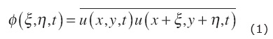
where the bar indicates time averaging. Under the assumption that the wavefield is stationary, Aki (1957) showed that the azimuthal average of the spatial autocorrelation function can be written as

where r and ψ are the polar coordinates defined
by

Aki (1957) showed that the azimuthal average of the spatial autocorrelation function,  (r) , is related to the power spectral density of the microtremor wavefield, Φ(ω), through
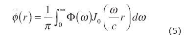
where J0 is the Bessel function of the first kind and zero order, and ω is angular frequency. This last equation also applies to the case of dispersive waves, and we need only substitute c(ω) for c. Assume now that we apply a bandpass filter to the records. The spectral density becomes

where P(ω0) is the power spectral density at frequency ω0 and δ( ) is Dirac's function. In this case, the azimuthal average of the spatial correlation function can be written as

Finally, Aki (1957) defined the autocorrelation coefficients, ρ(r, ω0), as
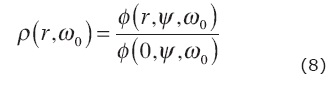
Because ρ(ω0) does not depend on the position (assumption of spatial stationarity), we can finally write the azimuthal average of the correlation coefficients as
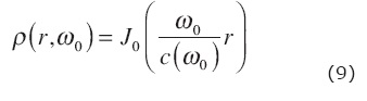
This last equation states that, if we are able to compute ρ(r, ω0) from microtremor measurements, we can estimate c (ω0). However, because the relation between the correlation coefficients and the phase velocity is non linear, an iterative inversion scheme is needed. In this paper we have used the inversion scheme described in detail in Chávez-García et al. (2005).
The derivation of the SPAC method was presented in great detail in Aki (1957) and Chouet et al. (1998) among others. Eq. (9) offers a way to compute the phase velocity, when we can estimate an azimuthal average of the spatial autocorrelation, for a fixed distance r. This was interpreted, starting with Aki (1965), as requiring several stations, distributed on a circle of radius r, with one station at the center of the circle. Naturally, if data recorded on several circles with different radii are available, an azimuthal average can be computed for each circle, and for a fixed frequency ω0, using r as independent variable.
The SPAC method has been used frequently to estimate a phase velocity dispersion of Rayleigh waves (e.g., Ferrazzini et al., 1991; Chouet et al., 1998; Yamamoto, 1998; Morikawa et al., 1998, 2004; Flores Estrella and Aguirre González, 2003; Chávez-García et al., 2005; Apostolidis et al., 2005, Margaryan et al., 2009). This method has also been complemented and/or compared with horizontal to vertical spectral ratios (HVSR) of microtremors (e.g., Roberts and Asten, 2005, 2007) with f-k (frequency-wavenumber method, e.g., Claprood and Asten, 2009), and with REMI, Refraction Microtremor method, proposed by Louie (2001) in Chávez-García et al. (2007). All those results showed SPAC to be very reliable. Once a dispersion curve is estimated, it is possible to invert it using standard methods (e.g., Herrmann, 1985) to obtain a 1D layered structure. The limitation is that the soil profile under the array of stations must be regular enough for a single surface wave mode to dominate the correlation functions. One of the limitations of the SPAC method was the need to use a circular array of stations. However, it has been shown (Ohori et al., 2002; Okada, 2003; Chávez-García et al., 2005) that it is possible to use of the SPAC method without the limitations imposed by the circular array. If the waves that form the microtremors propagate homogeneously in all directions, a single station pair samples all directions of propagation provided that temporal averaging is substituted for the azimuthal averaging. In that case, instead of deploying a circular array and estimating correlation coefficients for a distance equal to the radius of the circle, it is possible to analyse a single station pair as if the distance between the two stations were the radius of a circle of stations. This has increased significantly the applicability of the SPAC method. For example, Chávez-García et al. (2006) analysed successfully data recorded by a linear array. Ekström et al. (2009) used two-station SPAC to analyse data from USArray including 30,000 station pairs. In a more modest scale, we take advantage of this improvement in this paper.
If correlations in the frequency domain are useful, then because of the Fourier transform, they should also be useful in the time domain. However, the development of correlations in time domain to explore the subsoil has a different history. The first references are related to exploration seismology (e.g., Claerbout, 1968). Time domain correlation was rediscovered by helioseismologists (Duvall et al., 1993), before making its appearance in acoustics and seismology. In addition, time domain correlation of ambient noise has been the object of many theoretical studies that have been able to show its relation with the character of ambient noise and statistical properties of diffusive media. Weaver and Lobkis (2005) retrace briefly this history. The theoretical basis of the method and the conditions for its success have been the object of many papers (e.g., Campillo and Paul, 2003; Wapenaar, 2004; Snieder, 2004; Paul et al., 2005; Sabra et al., 2005; Roux et al., 2005; Bensen et al., 2007; Tsai, 2009, 2010). Time domain cross-correlation of microtremors, or seismic interferometry, is based on the relation that has been established between the cross-correlation function of a diffusive signal recorded at two sites and the time domain Green's function of the medium between the recording stations. Let us write the cross-correlation of microtremors (which can be shown to behave as a diffusive field) recorded at two locations as

where t is time, υi(r1, t) and υj(r2, t) are simultaneous recordings of microtremors at locations r1 and r2, T is the observation period and Cij is the cross-correlation computed between the two traces as a function of τ, the delay time. Among others, Sabra et al. (2005) have shown that

where Gij(r1; r2, t) is the time domain Green's function between the two locations. A review paper has been presented in Campillo (2006) and a useful compilation of 73 papers has been printed (Wapenaar et al., 2008). Results have been published from very small inter-station distances (5m in Chávez-García et al., 2006) to very large distances (thousands of km in Shapiro et al., 2005). Applications of this equation are abundant, from local or regional tomography (e.g., Shapiro et al., 2005; Yao et al., 2006; Kang and Shin, 2006; Moschetti et al., 2005; Yang et al., 2007; Prieto and Beroza, 2008) to volcano monitoring (e.g., Sens-Schönfelder and Wegler, 2006; Brenguier et al., 2007) and even to building response (Prieto et al., 2010).
The SPAC method and time domain cross-correlation are not completely independent methods. The data used is often the same and the operation (correlation) between traces is the same. The relation between the two methods has been anaysed in Chávez-García and Luzón (2005), Chávez-García and Rodríguez (2007), Yokoi and Margaryan (2008), Prieto et al. (2009), and Tsai and Moschetti (2010), among others. It is not the purpose of this paper to review that relation but we did compute time domain correlation functions, where we observed the emergence of the fundamental mode pulse for Rayleigh waves. In this paper we will only show an example of the equivalence of results obtained using cross-correlation in the frequency (SPAC method) and time domains (seismic interferometry). Some station pairs show a lack of correlation in both time and frequency domains, which we interpret in terms of lateral heterogeneity. When lateral variations occur over a distance larger than the size of the arrays, we may identify it through the comparison among the results for the different arrays. However, if the lateral heterogeneity occurs over a distance smaller than the distance between stations, no correlation is obtained in either frequency or time domains and the method fails.
Data
The studied region is located in the lake bed zone in Mexico City, close to the transition zone, along the trace of the Metro-A line (Figure 1). Triangular and linear arrays were deployed mainly along Ignacio Zaragoza avenue (Figure 2). Array aperture spanned a large range, from 10 to 1,960 m. Two different sensor types were used. Vertical sensors HV1 by Kinemetrics (5 s natural period) were used for the arrays smaller than 50 m. For these small arrays, HV1 sensors were installed forming a triangle and all three were cable connected to a single accelerograph. In this case, because the three signals were recorded by the same accelerograph, the sampling for all sensors was simultaneous. For larger triangles, we had to use independent recorders at each measurements point, and therefore had to check a common time base for all the records. We used GPS antennas to synchronize all recorders to GMT. If the accelerograph locks to the time signal received by the GPS antenna, then common time for all the records is guaranteed. There was only one triangle for which one of the accelerographs failed to lock its internal clock to the GPS time signal, and the record had to be discarded. For distances between stations of 60 m and larger, we used triaxial broad band sensors CMG40 by Guralp, able to record faithfully ground velocity down to 0.03 Hz, each one coupled to a different accelerograph. Ground vibration was recorded using K2 and Etna accelerographs by Kinemetrics.
A total of nine triangular arrays and two linear arrays were used to record microtremors. Table 1 gives the different sizes of the triangular and linear arrays used and Figure 2 shows their location. At each one of locations S1 to S6 (small green triangles in Figure 2), four or five different triangular arrays with side length from 10 to 45 m were used to record microtremors during 20 min for each array. Additional triangular arrays were deployed at locations A, B, and C (large green triangles in Figure 2). At positions A and B, 10 and 8 triangular arrays respectively were deployed, with side length between 10 and 500 m (Table 1). Figure 2 shows an additional large green triangle, labelled C, where only three triangular arrays (with side lengths of 200, 400, and 500 m) were deployed. All these arrays were used to record microtremors for 20 min for the smaller arrays and 30 min for the larger arrays.
Finally, two additional linear arrays (L1 and L2) were deployed using four stations for each one. Their location is shown with the blue and red lines in Figure 2. The distance between stations is given in Table 1. Array L1, solid blue line in Figure 2, had separation between stations varying between 100 and 500 m. Array L2, solid red line in Figure 2, had separation between stations going from 600 to 1,960 m. The two linear arrays recorded microtremors for one hour.
Frequency and time domain correlation functions were computed for all station pairs. Time windows selected for the analysis had an overlap of 50% of its width, which varied from 60 s for the smaller arrays (smaller than 50 m) and from 240 s for the larger arrays up to the complete record length (1,200 s for arrays S1 to S6, 1,800 s for the large triangles at locations A, B, and C, and 3,600 s for the linear arrays L1 and L2). The use of different window lengths allowed us to check the influence of the record length in the results of the correlation analysis. We verified that our final results did not depend on window length and that they were stable and independent of all processing parameters.
Results
Results for distances smaller than 50 m
Figure 3 shows an example of the correlation coefficients computed from the measurements at location A for distances between stations of 10, 20, 30, and 40 m. This figure shows the average correlation coefficients computed for each distance from the 180 time windows selected for the analysis (60 time windows of 60 s duration with 30 s overlap, for each one of the three station pairs at the same distance for each triangle). The vertical dashed lines in each frame indicate the frequency range for which the corresponding correlation coefficients resemble a J0 function. On the high frequency end of the plots, we observe that the correlation coefficients become almost flat at a smaller frequency as distance between stations increases: 15 Hz for 10 m, 8 Hz for 20 m, 6 Hz for 30 m, and 4 Hz for 40 m. At low frequencies we observe that correlation drops significantly at about 1 Hz in all four cases shown. This drop in correlation at low frequencies has also been observed by Chávez-García et al. (2006), Roberts and Asten (2007), and Claprood and Asten (2009). Roberts and Asten (2007) propose that the lowest frequency at which the correlation coefficients take the shape of a Bessel function coincides approximately with the peak values of the horizontal to vertical spectral ratios (HVSR) recorded at the same site. They speculate that high HVSR values imply low amplitudes of vertical component surface-wave motion, which results in the degradation of the correlation coefficients. Our results support this interpretation. As is shown below, for the small triangular arrays at location A, HVSR have a peak at frequencies between 0.4 and 1 Hz, coinciding with the trough in correlation at low frequencies of Figure 3. Similar results were obtained for all small (smaller than 50 m) triangular arrays, with the exception of array S6 as explained below.
Consider now an example of time domain correlation. Figure 4 shows average time domain correlation for all station pairs for the five triangles with size smaller than 50 m at location A (Figure 2), plotted at the corresponding distance between stations. They correspond then to the correlation coefficients shown in Figure 3. Again, each trace is the average for all possible station pairs at the corresponding distance. The pulse corresponding to the Rayleigh wave mode is clearly observed. The phase velocity of this pulse can be measured in Figure 4, it is about 100 m/s. Figure 5 shows the Fourier amplitude spectra of the four traces shown in Figure 4. The Rayleigh wave pulse apparent in Figure 4 has energy in the frequency band from 1 to 10 Hz, although the largest amplitudes occur between 1 and 4 Hz.
We inverted a phase velocity from the computed correlation coefficients at each location using eq. (9). Figure 6 shows the phase velocity dispersion curves derived from the small arrays (smaller than 50 m) with the exception of array S6. Figure 6 shows almost flat dispersion curves in the frequency range from 0.7 to 4 Hz. The frequency range for which results could be obtained is different for each measurement point. However, minimum (about 40 m) and maximum (about 140 m) wavelengths are similar for all cases. This was expected. The resolution of an array for correlation of microtremor measurements is a function of wavelength, as explained in detail in Henstridge (1979) and Chávez-García et al. (2005). The phase velocities that were obtained are also quite different among the different measurements points, from 60 to 220 m/s at 2 Hz. This result suggests significant lateral heterogeneity, with shear wave velocity of the topmost layer varying according to the location of the array. We can compare the frequency range for which a phase velocity could be estimated at point A in Figure 6 (between 1 and 3.4 Hz) with the frequency band for which a Rayleigh pulse is estimated using time domain correlation with the same microtremor records (shown in Figure 5). The lower frequency limit is the same, about 1 Hz. However, time domain correlation shows that the Rayleigh pulse has significant energy at least up to 10 Hz, whereas frequency domain results do not go above 3.4 Hz. The reason is that frequency domain correlation requires that the phase difference between the two records be unambiguously measured. This is not the case for wavelengths smaller than half the distance between the two stations, which violate the spatial version of the fundamental sampling theorem, as explained in detail in Chávez-García and Rodríguez (2007). However, the phase velocity estimated from the seismic section in Figure 5 coincides well with the results from SPAC for array A. The results from SPAC and time domain correlation are compatible.
Figure 6 does not show results for measurements at array S6. A 200 s window of raw microtremor data recorded at this array for 10 m distance between stations is shown in Figure 7, as an example of the records at that location. The records in this figure are dominated by very large amplitude transients, common to the three stations. We verified that these transients correspond to trucks and cars going by in the large Zaragoza Avenue; arrival time increases with distance to this avenue. Correlation between the traces is strongly affected by these signals which are certainly not aleatory (we can easily identify the same pulse in the three stations) and originate from a moving point source. The basic hypothesis of the SPAC method, waves propagating with equal power in all directions, is violated and no significant result could be obtained for this array.
Results for distances larger than 50 m
Let us consider now the results for station pairs separated a distance larger than 50 m. The results for these station pairs were not very good. The triangular arrays at locations A, B, and C included distances between 60 and 500 m (see Table 1). We computed correlations between the records in time and frequency domains, testing windows of different length for the analysis. We could not obtain significant correlation for any case. A possible reason for this lack of correlation could be that the microtremor records were not long enough. The recording time for the larger triangles at the locations of arrays A, B, and C was between 900 and 1,800 s.
In order to check whether the total length of microtremor recording was a problem, we planned two additional arrays, L1 and L2. These arrays were two lines of four stations each. The total length of these arrays was 500 m for L1 and 1,960 m for L2. One hour of microtremors were recorded simultaneously in the four stations of each linear array. We computed correlation coefficients for all station pairs for arrays L1 and L2 (the corresponding distances are given in Table 1) averaging results for windows of different duration selected from the records. We tested window durations between 240 and 3,600 s. An example of the results is given in Figure 8. This figure shows average correlation coefficients determined for four different station pairs from array L2. Each solid line in this figure corresponds to average correlation coefficients computed using a different number of windows of different duration, between 240 and 3,600 s. The good agreement among all five curves indicates that the window length has no significant effect on the results. Thus the lack of correlation observed for the triangular arrays at locations A, B, and C was not the result of the limited recording time. The correlation coefficients in Figure 8 are not similar to a J0 Bessel function, with the exception of a narrow frequency band (between 0.2 and 0.4 Hz) for the station pair at a distance of 600 m in Figure 8. Similar results were obtained for all station pairs from arrays L1 and L2. The correlation coefficients that were computed were not useful to invert a phase velocity dispersion curve based on eq. (9).
Even if the correlation coefficients from array L1 and L2 were inadequate for an inversion to obtain a phase velocity dispersion curve, for some station pairs, the observed correlation coefficients showed the expected behaviour, i.e., a shape similar to a J0 function, at least for small frequency windows, as shown for 600 m distance in Figure 8. Figure 9 shows the same correlation coefficients computed for the separation distance of 600 m for array L2. In this figure we have superposed a J0 function, manually fitted to the observations by changing the abscissa of each point while keeping the ordinates constant. This modified Bessel function is shown with solid green circles in Figure 9 in the frequency range 0.17 to 0.4 Hz. For each of these points, a phase velocity could be estimated from the comparison between the argument of the original J0 function and the value of the abscissa of that same point after being fitted to the observed correlation coefficients, using the relation between the argument of the Bessel function and the term œr/c. Using this non-standard procedure, we could obtain some estimates of phase velocity for distances of 100, 200, 300, and 500 m for array L1, and for 600 m for array L2, only for five out of the ten distances for which data were recorded in these arrays, and only five out of 22 distances larger than 50 m including measurements for locations A, B, and C.
The results for the five distances for which phase velocity dispersion could be estimated using this non-standard procedure are shown in Figure 10. The different symbols identify the corresponding station pair for which the phase velocity could be estimated. The frequency range of these estimates is very small, except for 100 m distance for array L1. Contrary to what was observed for small distances between stations, all the different estimates shown in Figure 10 are in good agreement among them, forming a single phase velocity dispersion curve. Phase velocity is almost constant at 75 m/s for frequencies larger than 0.8 Hz, in good agreement with a couple of the dispersion curves shown in Figure 6 for the smaller arrays. For frequencies smaller than 0.8 Hz, phase velocity in Figure 10 increases up to 450 m/s, indicating a significant velocity contrast below the soft surficial layer. However, because the phase velocity curve remains steep at low frequencies, it does not constrain the velocity below the sediments.
Velocity models
The phase velocity dispersion curves we estimated are consistent between our small and large arrays. However, although a significant velocity contrast below is clearly indentified, the results are unable to constrain the velocity of the deeper medium. Moreover, because the phase velocity estimates shown in Figure 10 were obtained using a manual fit of the Bessel function, they are less reliable than the phase velocities shown in Figure 6, obtained using a formal inversion scheme based on eq. (9). For these reasons, we have not tried to estimate a 1D layered model from the inversion of the phase velocity dispersion curves. Rather, we propose the model shown in Table 2, based on the phase velocity dispersion estimated in Figure 10. A single layer over a half space model is the simplest model that can fit the observed dispersion. This proposed model constrained the velocity of the soft layer to 75 m/s, to fit the Rayleigh phase velocity observed at frequencies larger than 1 Hz in Figure 10. The shear wave velocity of the half space must be larger than 500 m/s but is otherwise unconstrained. We took density values adequate for the soil layer and half space from Pérez-Cruz (1988). We computed phase velocity dispersion for the fundamental Rayleigh wave mode for the model in Table 2, varying the thickness of the layer until a reasonable fit was obtained. The computed dispersion curve is shown with a solid black line in Figure 10. Even if the model of Table 2 is not well constrained, the agreement between observed and computed phase velocity dispersion is quite good.

The simple model of Table 2 is also compatible with the phase velocity dispersion estimated from the smaller arrays. Figure 11 shows the estimates of phase velocity dispersion obtained from our small arrays (those shown in Figure 6) together with phase velocity dispersion curves computed for the fundamental mode of Rayleigh waves for models very similar to that in Table 2. The only change made was on the shear wave velocity of the soft layer. All other parameters of the model were kept constant. The shear wave velocity used for the layer is indicated next to each dispersion curve. We observe quite a good fit to the observed dispersion. This fit could be improved, were we to tweak the thickness of the soft layer but we do not think this to be useful at this stage because the model remains not well constrained. Figures 10 and 11 do show, however, that a model similar to that in Table 2 explains our observations and quantifies the lateral variation of the shear wave velocity of the topmost layer.
The results for our larger arrays are disappointing. At low frequencies the phase velocity dispersion curve is very steep, indicating a large impedance contrast at the base of the clay layer. That impedance contrast is the reason for the large amplification of seismic ground motion in the lake bed zone, which in a model such as that in Table 2 is equal to the impedance contrast between the layer and its substratum. Our results fail to constrain the shear wave velocity in the half-space. As explained in detail in Chávez-García (2011), if we cannot constrain the shear wave velocity below the soft sediments, we cannot compute the expected amplification. We expected that larger distances between stations would allow us to correlate waves propagating through the substratum. This is not the case.
The lack of correlation between our stations for distances larger than 600 m is similar to the results presented in Chávez-García and Quintanar (2010). Those authors computed correlation between stations separated from 5 to several hundred km. One of the arrays whose data they analysed crossed Mexico City. They observed a lack of correlation between stations closer than 10 km, even if the same stations showed good correlation with more distant stations. They ascribed the lack of correlation to strong lateral heterogeneities, expected for the thick volcanic sediment sequence below the clay layer in Mexico City basin. Chávez-García and Quintanar (2010) concluded that the heterogeneity of the deep structure of the Mexican Volcanic Belt inhibited the propagation of Rayleigh waves with wavelengths smaller than 9 km.
In the case of our results, Figure 10 shows a phase velocity of 400 m/s at 0.4 Hz. This implies a wavelength of 1 km, which is about the longest wave for which we obtain correlation among our stations. Considering together our results with those of Chávez-García and Quintanar (2010), we may conclude that there is a wavelength range between 1 and 9 km, for which no correlation is observed for microtremor records in Mexico City basin. However, information for this wavelength range is needed to constrain the shear-wave velocity structure of the volcanic sediments below the clay layers in the lake bed zone. This is a very significant problem and one that remains a challenge.
HVSR
Finally, we computed horizontal to vertical spectral ratios (HVSR) using the microtremor records where three-component ground motion was recorded. We estimated dominant period in the studied region from the large peaks observed in the HVSR. This is not incompatible with the interpretation of the records in terms of Rayleigh waves, as required by the SPAC method. It has been shown that HVSR gives stable results independently of the predominant propagation mode, body or surface waves (Chávez-García, 2009). Figure 12 shows the map distribution of dominant period obtained from our measurements. We observe significant variations, from 0. 8 s on Ignacio Zaragoza avenue up to almost 5 s for the measurements at the stations for the linear arrays L1 and L2. Dominant period varies rapidly over short distances. The dominant period value computed for the model of Table 2 (which does not correspond to a specific site but is mostly based on the results for array L1) is 3 s, in good agreement with the empirical values shown in Figure 12. We have superposed in this figure the dominant period curves shown in Figure 1, included in the Distrito Federal building code.
These curves are the result of the interpolation of available measurements, which are quite sparse in our studied region. This explains the large difference between our measurements of dominant period and the interpolated curves. These discrepancies suggest that additional measurements of dominant period are needed in the lake bed zone of Mexico City.
Conclusions
We have presented the results of subsoil exploration in the lake bed zone of Mexico City using correlation of microtremors recorded with arrays of stations. 46 independent triangular arrays and two linear arrays were installed with inter station distances between 10 m and almost 2 km. Microtremors were recorded for a few minutes at the smaller arrays and one hour at the larger arrays. Vertical components were analyzed using the SPAC method to recover Rayleigh wave dispersion. Our measurements allowed us to compute correlations of microtremors for a very wide range of distances between stations, from 10 m to 2 km.
Good results were obtained for distance between stations smaller than 50 m. The shallow velocity structure could be well determined from correlation analyses. Moreover, we obtained evidence of significant lateral heterogeneity in the clay layer. We showed that the velocities estimated using time domain cross-correlation, seismic interferometry, were compatible with the results from the SPAC method.
For distance between stations larger than 50 m, it was not possible to obtain good correlation. We only observed correlation coefficients similar to a Bessel function in small frequency ranges for five different distances (between 100 and 600 m) out of the 22 distance for which we recorded data. We demonstrated that this lack of correlation was not due to the duration of the microtremor records in the field. For those five different station pairs, we manually fitted a Bessel function to the narrow range of useful correlation coefficients and estimated from that phase velocity values in the frequency range from 0.3 to 1.4 Hz. The result shows that there is a significant impedance contrast at the base of the soft surficial sediments. However, our measurements are unable to constrain the velocity below those sediments. If we cannot determine the shear wave velocity of both sediments and basement, it is not possible to compute expected amplification. These results are disappointing. Our analysis indicates that the most likely cause is lateral heterogeneity of the sediments below the soft clay layers. Mexico City basin includes several km of volcanic sediments between the very soft clay layer at the surface in the lake bed zone and the limestone basement of the basin. Correlation between two stations requires that the medium, at the wavelength scale of distance between stations, be able to sustain Rayleigh waves. The large heterogeneity expected for volcanic sediments must affect surface wave propagation for wavelengths larger than 1 km in such a way that Rayleigh waves cannot be retrieved from frequency or time domain correlations. This conclusion is similar to those of Chávez-García and Quintanar (2010), who observed a lack of correlation in Mexico City for Rayleigh wavelengths smaller than 9 km. Our results show that we need an alternative method to investigate the subsoil structure for the wavelength range between 1 and 9 km.
We used the records obtained using triaxial sensors to estimate dominant period from horizontal to vertical spectral ratios. The results are compatible with those from correlation analyses. Our measurements provide reliable constraints on the variation of dominant period in the studied region. Dominant period changes significantly over short distances, similarly to the change of shear wave velocity of the topmost layers identified from correlation analyses. This was to be expected close to the edges of the ancient lake, where we anticipate rapid lateral variations in the subsoil structure. Our values for dominant period are quite different from the smooth curves included in Distrito Federal building code. The curves from the building code were interpolated from very few measurements in the studied region. This suggests that additional measurements of dominant period are needed in the lake bed zone of Mexico City. This is important because the building code specifies design spectra in terms of dominant frequency.
Finally, the correlation method, as any other method in Geophysics, has significant limitations. In the case of Mexico City, the determination of the velocity structure below the clay layer remains a challenge. That structure is important because it conditions the incident wavefield below the clay layer and is necessary to compute expected amplification.
Acknowledgements
We gratefully acknowledge the help of Antonio Valverde, Horacio Mijares, and Ricardo Vázquez Rosas for their help during the many days of field work. The comments by four anonymous reviewers were very helpful to improve our manuscript. Part of this research was supported by Instituto de Ingeniería, UNAM, through its fund for internal research projects 2010, project 0542.
Bibliography
Aki K., 1957, Space and time spectra of stationary stochastic waves, with special reference to microtremors, Bull. Earthquake Res. Inst. Univ. Tokyo, 25, 415-457. [ Links ]
Aki K., 1965, A note on the use of microseisms in determining the shallow structure of the earth's crust, Geophysics, 30, 665-666. [ Links ]
Apostolidis P., Raptakis D., Pandi K., Manakou M., Pitilakis K., 2005, Definition of subsoil structure and preliminary ground response in Aigion city (Greece) using microtremors and earthquakes, Soil Dyn. Earthq. Engng., 26: 922-940. [ Links ]
Bensen G.D., Ritzwoller M.H., Barmin M.P., Levshin A.L., Lin F., Moschetti M.P., Shapiro N.M., Yang Y., 2007, Processing seismic ambient noise data to obtain reliable broad-band surface wave dispersion measurements, Geophys. J. 169, 1239-1260, doi 10.1111/j.1365-246X.2007.03374.x. [ Links ]
Brenguier F., Shapiro N.M., Campillo M., Nercessian A., Ferrazzini V., 2007, 3D surface wave tomography of the Piton de la Fournaise volcano using seismic noise correlations, Geophys. Res. Lett., 34, L02305. [ Links ]
Campillo M., Paul A., 2003, Long range correlations in the diffuse seismic coda, Science, 299, 547-549. [ Links ]
Campillo M., 2006, Phase and correlation in 'random' seismic fields and the reconstruction of the Green's function, Pure Appl. Geophys., 163, 475-502. [ Links ]
Cárdenas M., Chávez-García F.J., Gusev A., 1997, Regional amplification of ground motion in central Mexico: results from coda magnitude data and preliminary modeling, J. Seism., 1, 341-355. [ Links ]
Chávez-García F.J., Bard P.-Y., 1993a, Gravity waves in Mexico City? I. Gravity perturbed waves in an elastic solid, Bull. Seism. Soc. Am., 83, 1637-1655. [ Links ]
Chávez-García F.J., Bard P.-Y., 1993b, Gravity waves in Mexico City? II. Coupling between an elastic solid and a fluid layer, Bull. Seism. Soc. Am., 83, 1656-1675. [ Links ]
Chávez-García F.J., Bard P.-Y. 1994, Site effects in Mexico City eight years after the September 1985 Michoacán earthquakes, Soil Dyn. Earthquake Eng., 13, 229-247. [ Links ]
Chávez-García, F.J. and L. Salazar (2002). Strong motion in central Mexico: a model based on data analysis and simple modelling, Bull. Seism. Soc. Am., 92, 3087-3101. [ Links ]
Chávez-García, F.J. y F. Luzon (2005). On the correlation of seismic microtremors, J. Geophys. Res., 110, B11313, doi: 10.1029/2005JB003671. [ Links ]
Chávez-García, F.J. (2007). Site effects: from observations and modelling to accounting for them in building codes, in K.D. Pitilakis (ed.) Earthquake Geotechnical Engineering, 4th International Conference of Earthquake Geotechnical Engineering - Invited lectures, vol. 6 of the series Geotechnical, Geological and Earthquake Engineering, ISBN: 978-1-40205892-9, ISSN 1573-6059, DOI 10.1007/9781-4020-5893-6, Springer, 53-72. [ Links ]
Chávez-García, F.J. and M. Rodríguez (2007). The correlation of microtremors: empirical limits and relations between results in frequency and time domains, Geophys. J. Int., 171, 657-664. [ Links ]
Chávez-García, F.J. (2009). Ambient noise and site response: from estimation of site effects to determination of the subsoil structure, en M. Mucciarelli, M. Herak y J. Cassidy (eds.) Increasing seismic safety by combining engineering technologies and seismological data, NATO Science for Peace and Security Series C: Environmental Security, ISBN 9781-4020-9193-3 Springer Science+Business Media B.V., 53-71. [ Links ]
Chávez-García, F.J. (2010). Site response at Mexico City. Progress made and pending issues, Joint Conference Proceedings, 7th International Conference on Urban Earthquake Engineering (7CUEE) & 5th International Conference on Earthquake Engineering (5ICEE), 3-5 de marzo, Tokyo Institute of Technology, Tokyo, Japón, 81-88. [ Links ]
Chávez-García, F.J. y L. Quintanar (2010). Velocity structure under the Trans-Mexican Volcanic Belt. Preliminary results using correlation of noise, Geophys. J. Int., 183, 1077-1086, doi: 10.1111/j.1365-246X.2010.04780.x. [ Links ]
Chávez-García, F.J. (2011). Site effects due to topography and to soft soil layers: progress made and pending issues. A personal perspective, conferencia estado-del-arte invitada en 5th International Conference on Earthquake Geotechnical Engineering, ISBN 978-956-7141-18-0, Chilean Geotechnical Society, 105-136. [ Links ]
Chávez-García, F.J., J. Ramos Martínez, and E. Romero-Jiménez (1995). Surface wave dispersion analysis in Mexico City, Bull. Seism. Soc. Am., 85, 1116-1126. [ Links ]
Chávez-García, F.J., M. Rodríguez, M. and W.R. Stephenson (2005). An alternative approach to the SPAC analysis of microtremors: exploiting stationarity of noise, Bull. Seism. Soc. Am., 95, 277-293. [ Links ]
Chávez-García, F.J., M. Rodríguez, and W.R. Stephenson (2006). Subsoil structure using SPAC measurements along a line, Bull. Seism. Soc. Am., 96, 729-736. [ Links ]
Chávez-García, F.J., T. Domínguez, M. Rodríguez, and F. Pérez (2007). Site effects in a volcanic environment: a comparison between HVSR and array techniques at Colima, Mexico, Bull. Seism. Soc. Am., 97, 591-604, doi: 10.1785/0120060095. [ Links ]
Chouet, B., G. DeLuca, G. Milana, P. Dawson, M. Martini, and R. Scarpa (1998). Shallow velocity structure of Stromboli volcano, Italy, derived from small-aperture array measurements of Strombolian tremor, Bull. Seism. Soc. Am., 88, 653-666. [ Links ]
Claerbout J.F., 1968, Synthesis of a layered medium from its acoustic transmission response, Geophysics, 33, 264-269. [ Links ]
Claprood, M. and M.W. Asten (2009). Initial results from spatially averaged coherency, frequency-wavenumber, and horizontal to vertical spectrum ratio microtremor survey methods for site hazard study at Launceston, Tasmania, Exploration Geophysics, 40, 132-142, Butsuri-Tansa, 62, 132-142, Mulli-Tamsa, 12, 132-142. [ Links ]
Duvall T.L., S.M. Jefferies, J.W. Harvey, and M.A. Pomerantz (1993). Time-distance helioseismology, Nature, 362, 430-432. [ Links ]
Ekström, G., G.A. Abers, and S.C. Webb (2009). Determination of surface-wave velocities across USArray from noise and Aki's spectral formulation, Geophys. Res. Lett., 36, L18301, doi:10.1029/2009GL039131. [ Links ]
Ferrazzini, V., K. Aki, and B. Chouet (1991). Characteristics of seismic waves composing Hawaiian volcanic tremor and gas-piston events observed by a near-source array, J. Geophys. Res., 96, 6199-6209. [ Links ]
Flores Estrella, H. and J. Aguirre-González (2003). SPAC: an alternative method to estimate earthquake site effects in Mexico City, Geofís. Int., 42, 227-236. [ Links ]
Furumura, T., and B. L. N. Kennett (1998). On the nature of regional seismic phases. III. The influence of crustal heterogeneity on the wavefield for subduction earthquakes: the 1985 Michoacan and 1995 Copala, Guerrero, Mexico earthquakes, Geophys. J. Int., 135, 1060-1084. [ Links ]
Henstridge, D.J. (1979). A signal processing method for circular arrays, Geophysics, 44, 179-184. [ Links ]
Herrmann, R.B. (1985). Computer programs in Seismology, 8 vols., Saint Louis University. [ Links ]
Iida, M. (1999). Excitation of high-frequency surface waves with long duration in the Valley of Mexico, J. Geophys. Res., 104, 7329-7345. [ Links ]
Kang, T.S. and J.S. Shin (2006). Surface-wave tomography from ambient seismic noise of accelerograph networks in southern Korea, Geophys. Res. Lett., 33, L17303, doi:10.1029/2006GL027044. [ Links ]
Kawase, H. and K. Aki (1989). A study on the response of a soft soil basin for incident S, P, and Rayleigh waves with special reference to the long duration observed in Mexico City, Bull. Seism. Soc. Am., 79, 1361-1382. [ Links ]
Lermo J. and F.J. Chávez-García (1993). Site effect evaluation using spectral ratios with only one station, Bull. Seism. Soc. Am., 83, 1574-1594. [ Links ]
Lermo, J. and F.J. Chávez-García (1994). Site effect evaluation at Mexico City: dominant period and relative amplification from strong motion and microtremor records, Soil Dyn. & Earthq. Engrg., 13, 413-423. [ Links ]
Louie, J.N. (2001). Faster, better: shear-wave velocity to 100 meters depths from refraction microtremor arrays, Bull. Seism. Soc. Am., 91, 347-364. [ Links ]
Margaryan, S., T. Yokoi, and K. Hayashi (2009). Experiments on the stability of the spatial autocorrelation method (SPAC) and linear array methods and on the imaginary part of the SPAC coefficients as an indicator of data quality, Explor. Geophys., 40, 121-131; Butsuri-Tansa, 62, 121-131; Mulli-Tamsa, 12, 121-131. [ Links ]
Morikawa, H., K. Toki, S. Sawada, J. Akamatsu, K. Miyakoshi, J. Ejiri, and D. Nakajima (1998). Detection of dispersion curves from microseisms observed at two sites, in The effects of surface geology on seismic motion; Proc. of the 2nd. Intl. Symp. on the effects of surface geology on seismic motion, K. Irikura, K. Kudo, H. Okada, and T. Sasatani (Editors) 2, 719-724. [ Links ]
Morikawa, H., S. Sawada, and J. Akamatsu (2004) . A method to estimate phase velocities of Rayleigh waves using microseisms simultaneously observed at two sites, Bull. Seism. Soc. Am., 94, 961-976. [ Links ]
Moschetti, M.P., M.H. Ritzwoller, and N.M. Shapiro (2005) . California surface wave tomography from ambient seismic soise: tracking the progress of the USArray transportable network, EOS, Trans. Am. geophys. Un., 86(52), Fall Meet. Suppl., Abstract S31A-0276. [ Links ]
Ohori M., A. Nobata, and K. Wakamatsu (2002). A comparison of ESAC and FK methods of estimating phase velocity using arbitrarily shaped microtremor arrays, Bull. Seism. Soc. Am., 92, 2323-2332. [ Links ]
Okada H. (2003) The microtremor survey method, Soc. of Expl. Geophys. of Japan, translated by K. Suto, Geophys. Monograph Series No. 12, Soc. of Expl. Geophys., Tulsa. [ Links ]
Ordaz, M. and S.K. Singh (1992). Source spectra and spectral attenuation of seismic waves from Mexico earthquakes, and evidence of amplification in the hill zone of Mexico City, Bull. Seism. Soc. Am., 82, 24-43. [ Links ]
Paul, A., M. Campillo, L. Margerin, and E. Larose (2005). Empirical synthesis of time-asymmetrical Green's functions from the correlation of coda waves, J. Geophys. Res., 110, B08302, doi:10.1029/2004JB003521. [ Links ]
Pérez-Cruz, G.A. (1988). Estudio sismológico de reflexión del subsuelo de la Ciudad de México, M.Eng. Thesis, Facultad de Ingeniería, UNAM, 81 pp. [ Links ]
Prieto, G.A. and G.C. Beroza (2008). Earthquake ground motion prediction using the ambient seismic field, Geophys. Res. Lett., 35, L14304, doi:10.1029/2008GL034428. [ Links ]
Prieto, G.A, J.F. Lawrence, and G.C. Beroza (2009). Anelastic Earth structure from the coherency of ambient seismic field, J. Geophys. Res., 114, B07303, doi:10.1029/2008JB006067. [ Links ]
Prieto, G.A., J.F. Lawrence, A.I. Chung, and M.D. Kohler (2010). Impulse response of civil structures from ambient noise analysis, Bull. Seism. Soc. Am., 100, 2322-2328, doi: 10.1785/0120090285. [ Links ]
Roberts, J.C. and M.W. Asten (2005). Estimating the shear velocity profile of Quaternary silts using microtremor array (SPAC) measurements, Exploration Geophysics, 36, 34-40, Butsuri-Tansam 58, Mulli-Tamsa, 8. [ Links ]
Roberts, J.C. and M.W. Asten (2007). Further investigation over Quaternary silts using the spatial autocorrelation (SPAC) and horizontal to vertical spectral ratio (HVSR) microtremor methods, Exploration Geophysics, 38, 175-183. [ Links ]
Roux, P., K.G. Sabra, W.A. Kuperman, and A. Roux (2005). Ambient noise correlations in free space: theoretical approach, J. acoust. Soc. Am., 117, 79-84. [ Links ]
Sabra, K.G., P. Gerstoft, P. Roux, W.A. Kuperman, and M.C. Fehler (2005). Extracting timedomain Green's function estimates from ambient seismic noise, Geophys. Res. Lett., 32, L03310, doi:10.1029/2004GL021862. [ Links ]
Seed, H.B., M.P. Romo, J.I. Sun, A. Jaime, and J. Lysmer (1988). Relationships between soil condiriont and earthquake ground motion, Earthquake Spectra, 4, 687-729. [ Links ]
Sens-Schönfelder, C. and U. Wegler (2006). Passive image interferometry and seasonal variations of seismic velocities at Merapi Volcano, Indonesia, Geophys. Res. Lett., 33, L21302. [ Links ]
Shapiro, M.N., M. Campillo, A. Paul, S.K. Singh, D. Jongmans, and F.J. Sánchez-Sesma (1997). Surface wave propagation across the Mexican Volcanic Belt and the origin of the log-period seismic-wave amplification in the Valley of Mexico, Geophys. J. Int., 128, 151-166. [ Links ]
Shapiro, N.M., K.B. Olsen, and S.K. Singh (2001). Evidence of the dominance of highermode surface waves in the lake-bed zone of the valley of Mexico, Geophys. J. Int., 147, 517-527. [ Links ]
Shapiro, N.M., M. Campillo, L. Stehly, and M.H. Ritzwoller (2005). High-resolution surface-wave tomography from ambient seismic noise, Science, 307, 1615-1618, doi:10.1126/ science.1108339. [ Links ]
Singh, S.K., E. Mena, and R. Castro (1988). Some aspects of the source characteristics and ground motion amplifications in and near Mexico City from acceleration data of the September, 1985, Michoacan, Mexico earthquakes, Bull. Seism. Soc. Am., 78, 451-477. [ Links ]
Singh, S.K., R. Quaas, M. Ordaz, F. Mooser, D. Almora, M. Torres, and R. Vásquez (1995). Is there truly a 'hard' rock site in the Valley of Mexico?, Geophys. Res. Lett., 22, 481-484. [ Links ]
Snieder, R. (2004). Extracting the Green's function from the correlation of coda waves: a derivation based on stationary phase, Phys. Rev. E, 69, doi:10.1103/PhysRevE.69.046610. [ Links ]
Tsai, V.C. (2009). On establishing the accuracy of noise tomography travel-time measurements in a realistic medium, Geophys. J. Int., 178, 1555-1564, doi: 10.1111/j.1365-246X.2009.04239.x. [ Links ]
Tsai, V.C. (2010). The relationship between noise correlation and the Green's function in the presence of degeneracy and the absence of equipartition, Geophys. J. Int., 182, 1509-1514, doi: 10.1111/j.1365-246X.2010.04693.x. [ Links ]
Tsai, V.C. and M.P. Moschetti (2010). An explicit relationship between time-domain noise correlation and spatial autocorrelation (SPAC) results, Geophys. J. Int., 182, 454-460, doi: 10.1111/j.1365-246X.2010.04633.x. [ Links ]
Wapenaar, K. (2004). Retrieving the elastodynamic Green's function of an arbitrary inhomogeneous medium by cross correlation, Phys. Rev. Lett., 93(25), Article 254301. [ Links ]
Wapenaar, K., D. Draganov, and J.O.A. Robertsson (eds.) (2008). Seismic interferometry: history and present status, SEG Geophysics Reprint Series No. 26, Tulsa, Oklahoma. [ Links ]
Weaver R.L. and O.I. Lobkis (2005). Fluctuations in diffuse field-field correlations and the emergence of the Green's function in open systems, J. Acoust. Soc. Am., 117, 3432-3439. [ Links ]
Yamamoto, H. (1998). An experiment for estimating S-wave velocity structure from phase velocities of Love and Rayleigh waves in microtremors, in The effects of surface geology on seismic motion; Proc. of the 2nd. Intl. Symp. on the Effects of Surface Geology on Seismic Motion, K. Irikura, K. Kudo, H. Okada, and T. Sasatani (Editors), Rotterdam, Balkema, 2, 705-71. [ Links ]
Yang, Y., M.H. Ritzwoller, A.L. Levshin, and N.M. Shapiro (2007). Ambient noise Rayleigh tomography across Europe, Geophys. J. Int., 168, 259-274, doi: 10.1111/j.1365-246X.2006.03203.x. [ Links ]
Yao, H., R.D. van der Hilst, and M.V. De Hoop (2006). Surface-wave array tomography in SE Tibet from ambient seismic noise and twostation analysis: I—Phase velocity maps, Geophys. J. Int., 166, 732-744. [ Links ]
Yokoi, T. and S. Margaryan (2008). Consistency of the spatial autocorrelation method with seismic interferometry and its consequence, Geophys. Prospecting, 56, 4351,451, doi:10.1111/j.1365-2478.2008.00709.x. [ Links ]

