Original paper

 

Structural pattern of subsidence in an urban area of the southeastern Mexico Basin inferred from electrical resistivity tomography

 

Claudia Arango–Galván¹*, Brenda De la Torre–González², René E. Chávez–Segura¹, Andrés Tejero–Andrade², Gerardo Cifuentes–Nava¹ and Esteban Hernández–Quintero¹

 

¹ Instituto de Geofísica, Universidad Nacional Autónoma de México, Ciudad Universitaria, Delegación Coyoacán, 04510, México D.F., México. *Corresponding author: claudiar@geofisica.unam.mx

² Departamento de Geofísica Facultad de Ingeniería Universidad Nacional Autónoma de México Ciudad Universitaria Delegación Coyoacán, 04510 México D.F., México.

 

Received: August 6, 2010.
Accepted: June 3, 2011.
Published on line: September 30, 2011.

 

Resumen

La mayor parte de la zona urbana de la Cuenca de México está construida sobre los sedimentos de los antiguos lagos de Chalco, Xochimilco, México, Texcoco, Xaltocan y Zumpango, lo cual ofrece poca resistencia a las obras civiles que se asientan sobre ella. Adicionalmente, los requerimientos para el abastecimiento de agua potable para la población han generado la sobreexplotación de los acuíferos, exacerbando el fenómeno de subsidencia y el colapso de edificios, unidades habitacionales y caminos. Con la finalidad de entender el patrón de fracturamiento, así como su ubicación, se implementó un estudio geofísico con la técnica de tomografía de resistividad eléctrica en una zona poblada ubicada al sureste de la Cuenca de México.

Cinco secciones bidimensionales fueron calculadas a partir de los datos de resistividad adquiridos. En todas ellas fue posible identificar un horizonte resistivo discontinuo probablemente compuesto por algún material ígneo extrusivo. Las discontinuidades de este horizonte pueden ser relacionadas con grietas o fracturas identificadas con antelación sobre la superficie y que afectan obras civiles.

Además, un modelo tridimensional de resistividad fue calculado. La imagen 3D coincide con los resultados obtenidos de los modelos 2D, mostrando una capa resistiva con discontinuidades laterales. El patrón estructural de las fracturas inferido presenta una dirección preferencial NW–SE, el cual también genera el proceso de subsidencia en la zona, producido por la sobreexplotación del acuífero.

Palabras clave: subsidencia, tomografía de resistividad eléctrica, modelo bidimensional, modelo tridimensional, Cuenca de México, patrón estructural.

 

Abstract

Most of the urban area in the Basin of Mexico is underlain by sediments of the former lakes of Chalco, Xochimilco, Mexico, Texcoco, Xaltocan and Zumpango, which offer poor foundation conditions for buildings. Water supply requirements have led to overexploitation of the aquifers, and the increased exacerbating the rate of subsidence causes housing units and roads to deteriorate. In order to understand the location of the cracking and fracturing pattern, a geophysical study using electrical resistivity tomography was performed in a populated zone of the southeastern Mexico Basin. Five two–dimensional resistivity profiles were acquired. Discontinuities in the resistive horizon (probably in extrusive igneous material) were identified. The discontinuities could be related to cracks and fractures observed on the surface which had previously damaged housing construction.

A three–dimensional resistivity profile was also obtained. The 3D image confirms results obtained from 2D models, and shows a resistive layer with lateral discontinuities. The inferred fracture pattern has a preferential NW–SE direction, related to the a subsidence process produced by overexploitation of the aquifer in the area.

Key words: subsidence, electrical resistivity, tomography, two–dimensional model, three–dimensional model, Mexico basin, structural pattern.

 

Introduction

In recent years, soil subsidence has dramatically increased in the eastern Mexico Basin. It is especially notificable in densely populated areas, because of damage to housing infrastructure, and main roads.

Most of the urban area the basin of Mexico is built on sediments of the former lakes of Chalco, Xochimilco, Mexico, Texcoco, Xaltocan and Zumpango.

Saturated sandy clay in these sediments have a weak resistance to vertical loads. Some studies describe these materials as highly compressive because of high water content, more than 400% (e.g., Marsal and Mazari, 1959; Díaz–Rodríguez, 2006). The geological composition of sediments in the basin of Mexico is very diverse, from volcanic and lacustrine sediments to lava flows and conglomerates. In addition, the increasing need of water supply for the population in the basin, around 22 million inhabitants, has led to overexploitation of the main groundwater aquifers. This problem adds to the effect of physical properties of the subsoil like compressibility, resistance, cohesion, and low bearing capacity of soils. (Ovando–Shelley et al., 2003).

Clay sediments are sensitive to subsidence because their mechanical properties are directly linked to water content (Auvinet, 1981; Auvinet and Arias, 1991; Lermo and Chávez–García, 1994). Many fractures and cracks developed due to groundwater extraction, leading to failures in structures and settlement (Auvinet and Arias, 1991; Auvinet, 2008). The high rate of subsidence threatens the population and infrastructure in the area (Auvinet, 2009).

Subsidence features have traditionally been studied using geological and geotechnical techniques, such as mechanical soundings and boreholes (e.g., Auvinet, 1981; Auvinet, 2008; Méndez et al., 2008; Ovando–Shelley and Romo, 1992; Santoyo et al., 2005); but they are limited to narrow areas because of the heterogeneity of the sediments. Geophysical methods can also be applied to gain some insight into the impact (e.g., Lermo and Chávez–García, 1994; Díaz–Molina, 2001; Pacheco, 2007). Indirect techniques allow mapping wider areas without disturbing the subsoil, besides allowing the identification of structures not visible at the surface.

Electrical resistivity tomography (ERT) allows determining the electrical resistivity distribution of the subsurface, which is highly sensitive to many factors such as mineral composition, changes in porosity, and permeability (Meju, 2002). It has extensively been applied to mapping near surface features in urban zones with many different objectives such as geotechnical, environmental and archaeological prospecting (e.g., Chávez et al., 2001; Tejero et al., 2002; Shevnin et al., 2003; Cardarelli et al., 2010).

In this work of the ERT technique has been applied to the study of subsidence in a densely populated area. In the eastern Mexico Basin, a multi–family residential zone near the La Paz County (Estado de México) and Iztapalapa Country (Distrito Federal) boundary has been surveyed (Figure 1). The main objectives of this work are: 1) to determine the distribution of the anomalies in the subsurface system, and 2) to correlate them with the fracture and crack pattern identified on surface.

 

Geological setting

The Mexico Basin is located in a belt of recent volcanic structures. The formation of these volcanoes is attributed to an existing zone of weakness through which the magma has risen (Alaniz–Álvarez and Nieto–Samaniego, 2005). The Mexico Basin is located in the central Trans–Mexican Volcanic Belt (TMVB), a highly complex tectonic zone. Mexico basin contains andesitic and basaltic flows as well as poorly consolidated lacustrine sediments, tuffs and tephra. The study area is located on Cenozoic sediment accumulation in a floodplain close to Caldera volcano (Figure 1) (Tapia–Varela and López–Blanco, 2001). A group of volcanic structures with a west–east alignment surrounds this area. These volcanoes are part of Santa Catarina range, the youngest volcanic event in the geological history of the Basin (end of Pleistocene and Holocene).

According to Mooser (1975), the origin of the Santa Catarina range is related to shearing in a fault system that controls structures like Yuhualixqui volcano. De Cserna et al. (1988) confirm this theory by showing that the main structural control of the Santa Catarina range is a normal fault with a N75–80°E direction. Santa Catarina range is the end point of volcanic migration from west to east. La Caldera volcano, is the result of a phreatic–magmatic event, surrounded by lava flows from the Guadalupe volcano.

Figure 1 shows the geological setting of the study area. The area of interest is on lacustrine deposits, comprising clastic sediments and pyro–clastic products related to the activity of Po–pocatépetl volcano and Chichinautzin volcanic range. The thickness of these lacustrine sediments varies, from 300 m towards the central portion of the basin (Mexico City, Texcoco and Chalco) up to 30 m near the margins of the basin (Vázquez Sánchez and Jaimes–Palomera, 1989).

This plain has been widely studied, several authors (e.g., Mooser, 1975; DeCserna et al., 1988; Vázquez–Sánchez and Jaimes–Palomera, 1989; Lugo–Hubp et al., 1994) have determined by means of wells alternating materials, interstratifications of clay, alluvial and volcanic materials; some of these wells have been located at the northern edge of the Sierra Chichinautzin and around Sierra de Santa Catarina. The pyroclastic materials belong to the Chichinautzin formation (Vázquez–Sánchez and Jaimes–Palomera, 1989; Lugo–Hubp et al. 1994), which are 4,800–4,600 years old. This means that such a range was formed during the Late Pleistocene to Holocene. The lacustrine deposits have taken place due to obstruction of the last drainage of the basin of Mexico, caused by the intense activity of the Sierra Chichinautzin (Vázquez–Sánchez and Jaimes–Palomera, 1989).

Marsal and Mazari (1959) proposed that materials that constitute the basin of Mexico could be classified in three main geotechnical zones. This work was the first successful attempt to classify the subsoil according to its mechanical properties and composition. In fact, current building regulations are based on it (GDF, 2004). According to this classification, the lacustrine zone has poorly consolidated sediments, part of an ancient lake, featured by a high compressibility. Some small layers or lenses of similar composition showing a higher compaction can be intercalated modifying abruptly the mechanical properties in short spaces. Heterogeneous layers mainly compose the transition zone. Lenses from lacustrine materials (different grain sizes) can be intercalated. Its bearing capacity is variable; therefore it is susceptible to differential subsidence and poor ground stability. Finally, harder materials like tuffs, lava flows and pumice compose the hills zone, which has a high bearing capacity and negligible compressibility. This zone shows favorable conditions for building construction. The studied area is found on clastic sediments and pyroclastic products corresponding to the transition zone (Tapia–Varela y López–Blanco, 2001).

 

ERT data surveys

The applicability of ERT to fractures and cracks mapping has been successfully tested (e.g., Hao et al., 2002; Tejero et al., 2002; Kim et al., 2007; Cardarelli et al., 2010; Ha et al., 2010; García–Moreno and Mateos, 2010). As we have mentioned, imaging electrical resistivity distribution of the subsurface could be helpful to determine changes in the intrinsic properties of the rocks and sediments like, permeability and porosity that are modified by the presence of a discontinuity like a fault, a fracture or a crack. The ERT uses direct current as a source; the thus generated electric potential is detected between two points by two electrodes at different distances on the ground surface and provides information about both lateral and vertical resistivity distribution in subsurface. The apparent resistivity is obtained from these potential measurements. The final image of the true resistivity distribution is computed using an inversion algorithm developed by Loke and Barker(1996).

 

Data acquisition and processing

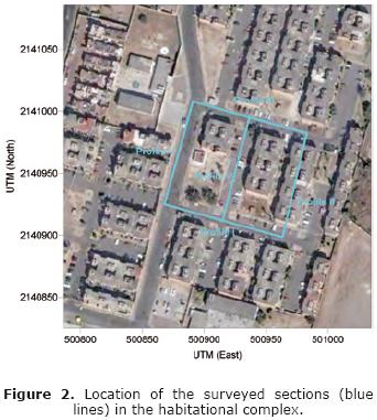
In this work, five 85 m long profiles were acquired around the affected buildings in the residential zone. Profiles I and III were carried out with NW–SE orientation and the profiles II, IV and V were acquired in NE–SW direction (Figure 2). A dipole–dipole array was employed with an interelectrodic distance of 5 m, using a total of 18 electrodes. This array was chosen because it is very sensitive to horizontal changes in resistivity; an expected behavior in cracks and fractures. However, this array shows a lower capability to detect vertical changes. In this sense, it is a good option to identify cracking and fracturing in a layer that does not show a significant change in its lithological composition. Depth of investigation of the array will depend on both distance between electrodes and the number of measured levels. In this study, almost 18% of the total length of the profiles was reached in depth penetration as has been reported by Edwards (1977) for dipole–dipole arrays. The equipment used in the acquisition was a console Sting R1 Swift–IP unit by AGI, 18 cooper electrodes 20 inches length and 24–channel automatic cables. The material, where electrodes were driven into, was a saturated clayed soil, which helped to reduce the contact resistance. Also, each electrode was wet with a salt–water solution in order to improve the electrode contact. In general, data quality was quite good. Nevertheless, some measurements (less than 5%) were removed because of high levels of noise. As it has been widely discussed in some studies, terrain topography is an effect that must be considered during the inversion process (e.g., Tsourlos et al., 1999; Xu et al., 2002; Wu, 2005; Mendoza and Dahlin, 2008; Erdogan et al., 2008; Vachiratienchai et al., 2010). This effect could perturb the current distribution in the subsurface and perturb the measured resistivity data and it is depend on the type of resistivity array (Tsourlos et al., 1999). However in this study, the topographic correction was not applied since the maximum gap elevation between the ends of the profiles was less than 60 centimeters and the expected disturbances are not large enough to affect the subsurface resistivity distribution at the working scale.

 

Results

2D models

As a preliminary processing, acquired data were inverted into five two–dimensional models (Figure 3). As we have already mentioned, true resistivity images were computed using a 2D inversion algorithm (Loke and Barker, 1996). The used inversion scheme was based on the regularized least–squares optimization; frequently called smooth inversion because it shows a smooth variation in the subsurface resistivity distribution (Loke et al., 2003). We used this scheme because the supposed geological structure does not show abrupt resistivity changes or sharp boundaries. On the contrary, we expected that this structure shows a gradual change in the resistivity values along the survey lines. The maximum depth reached by the geoelectrical sections was approximately 15 m.

All profiles show a common feature due to electrode watering effects. We can identify a superficial conductive layer located within the first 2 m deep. The watering effect saturated the upper part of the section, which is shown as this shallow conductive horizon in the geoelectrical models (Figure 3).

In profile I, it can be identified a resistive layer (>2,000 Ohm.m), to a depth of 3 m, which has a thickness of 10 m, approximately. The most important identified feature in this horizon is a lack of lateral continuity around 30 m, which depicted a weak structural zone. At the top of this layer, we can observe some depressions around fiducials 25, 47 and 64 m (red arrows). These structures are probably related to subsidence as observed on surface. In profile III, which is parallel to profile I, it is observed almost the same resistivity distribution; however, the bottom of the resistive layer is detected at depth of 15 m.

In profile II, the resistive horizon identified in profiles I and III presents a lower resistivity value (around 1,000 Ohm.m). This resistive layer is thinner with its bottom at around 12 m deep. A lateral discontinuity, at fiducial 50 m, is depicted by lower resistivity values (>500 Ohm.m) is probably related to a fracture.

In profiles IV and V, the thickness of this resistive material increases up to 13 m. In both sections the lateral discontinuity detected around 50 m is identified but is more evident in profile IV.

Figure 4 shows a 3–D composition of the five 2–D sections. By connecting the lateral discontinuities according to their position in each profiles we obtain the fracture pattern. Also, we can associate the major fracture exposed on surface with depressions detected on top of the resistivity layer in sections I and IV.

Pseudo 3D model

Although the original objective of this paper was to report two–dimensional sections, the relative location of the acquired profiles made it possible to obtain a geoelectrical model using a three–dimensional inversion algorithm (Li and Oldenburg, 1992; White et al, 2003). Nevertheless, this pseudo three–dimensional model has certain limitations, mainly due to distance between acquired profiles (80 m between profiles I and III; 40 m between profiles II, IV and V), which means that distribution of allocated points is not homogeneous.

The aim of inverting for a pseudo 3–D model was trying to detect if the three–dimensional resistivity distribution allowed us to map any preferential direction of fracture pattern. Although this was already inferred from two–dimensional models, we wanted to confirm the fracture pattern of the subsurface.

As it has been said, the data acquisition was not planned to build a real 3–D model. For this situation, we decided to compute a pseudo 3–D model using the two–dimensional available information. Despite, this process was difficult to implement because the distance between profiles was too large and we had interpolation problems during inversion, we obtained a consistent pseudo 3–D model well correlated with 2–D models and the geological evidences in the zone.

Final pseudo 3–D model is shown in Figure 5. The electrical resistivity distribution observed in this image coincides with the main characteristics detected in two–dimensional sections. However, some differences can be identified. Along section IV, the low resistivity values related to electrode effect are more evident than in the two–dimensional geoelectrical model. Despite this feature, the depicted anomalies in two–dimensional sections are emphasized in the pseudo three–dimensional model. It is possible to visualize three different trends, which clearly interrupt the main resistive bodies identified in the image. The first discontinuity direction splits up the resistive layer in a mean NS direction. The second anomalous trend separates the resistive layer in EW direction, coinciding with the discontinuity identified in profiles II, IV and V around fiducial 50 m. Finally, the third trend is located in the middle section of the inverted model of resistivities. It is interrupting up the resistive horizon in NE–SW direction. This last one coincides with the location of the main fracture observed on surface.

 

Conclusions

This geoelectrical study provides a fairly accurate subsurface image of the fractures affecting the studied zone. Five two–dimensional profiles and a pseudo three–dimensional model were computed using 2D and 3D algorithms respectively. Some main geoelectrical features can be inferred from these results:

1) A shallow low resistive layer was identified in the first 3 m depth along all two–dimensional sections. This effect is interpreted to be caused by the salt–water solution used to wet the electrodes.

2) Beneath this layer a high resistive horizon was detected showing lateral discontinuities. The resistive values of this layer are becoming higher through the western part of the studied zone.

3) The high values of resistivity may be due to the nature of the material; it can be extrusive igneous material produced by volcanic structures located near the study zone.

4) The anomalous lateral discontinuities identified in this layer coincide with cracks and fractures identified on surface.

According to the geoelectrical models, the main features inferred are due to the presence of three main alignments where the resistive body shows discontinuities, likely related to fracture zones. These alignments are coincident with the already reported faulting and also with the direction of the exposed crack detected in the study area. These discontinuities seem to be caused by two main factors: a) the overexploitation of the aquifers in the area, causing a loss of cohesiveness in the sediments and eventually generates a collapse; b) the proximity to volcanic structures, which are controlling the faulting regime in the sediments because of the presence of major tectonic faults in deeper zones.

This study contributes to get an insight of the subsidence phenomena in the area, and the obtained results confirm that the zone shows a high risk of subsidence collapse. Therefore, this type of studies helps to authorities to focus on the most susceptible zones in order to take appropriate measures to prevent risks.

 

Acknowledgments

We would like to thank the Faculty of Engineering UNAM, for supplying equipment. We also thank our students for their help during the fieldwork. We are indebted to the reviewers for their comments to improve the manuscript.

 

Bibliography

Alaniz–Álvarez S.A., Nieto–Samaniego A.F., 2005, El sistema de fallas Taxco–San Miguel de Allende y la Faja Volcánica Transmexicana, dos fronteras tectónicas del centro de México activas durante el Cenozoico. Boletín de la Sociedad Geológica Mexicana, LVII (1), 65–82.         [ Links ]

Auvinet G., 1981, Agrietamiento de las arcillas del valle de México. Informe Técnico del Instituto de Ingeniería, UNAM, a la Comisión del Lago de Texcoco, México, D.F.         [ Links ]

Auvinet G., Arias A.,1991, Propagación de grietas. Memorias del Simposio sobre Agrietamiento de Suelos, Sociedad Mexicana de Mecánica de Suelos, México, D.F., 21–32.         [ Links ]

Auvinet G., 2008, Fracturamiento de suelos: Estado del Arte. Memorias de la XXIV Reunión Nacional de Mecánica de Suelos, Vol. "Conferencias temáticas: Avances recientes". Aguascalientes, México, 299–318.         [ Links ]

Auvinet G., 2009, Land subsidence in Mexico City. Proceedings, ISSMGE TC36 workshop "Geotechnical engineering in urban areas affected by land subsidence; The cases of Mexico City, Bangkok and other large cities". México, D.F. ISBN 978–968–5350–24–2.         [ Links ]

Cardarelli E., Cercato M., Cerreto A., Di Filippo G., 2010, Electrical resistivity and seismic refraction tomography to detected buried cavities. Geophysical Prospecting, 58, 685695.         [ Links ]

Chávez R.E., Cámara M.E., Tejero A., Barba L., Manzanilla L., 2001, Site characterization by geophysical methods in the archaeological zone of Teotihuacan, Mexico. Journal of Archaeological Science, 28: 1,265–1,276.         [ Links ]

De Cserna Z., De la Fuente–Dunch M., Palacios–Nieto M., Triay L., Mitre–Salazar L.M., Mota–Palomino R., 1988, Estructura geológica, gravimétrica, sismicidad y relaciones neotectónicas regionales de la Cuenca de México. Boletín del Instituto de Geología, 104, 71 pp.         [ Links ]

De la Teja M., Sánchez E., Moctezuma M., De los Santos J., 2002, Carta Geológico–Minera Ciudad de México E14–2, Estado de México, Tlaxcala, D.F., Puebla, Hidalgo y Morelos. Servicio Geológico Mexicano.         [ Links ]

Díaz–Molina O., 2001, Determinación de zonas de riesgo geológico–ambiental en la Cuenca de México mediante sensores remotos y radar de penetración somera. Tesis de Licenciatura. Facultad de Ingeniería, UNAM. México, D.F. 89 pp.         [ Links ]

Díaz–Rodríguez J.A., 2006, Los suelos lacustres de la Ciudad de México. Revista Internacional de Desastres Naturales, Accidentes e Infraestructura Civil, 6(2):111–129.         [ Links ]

Edwards L.S., 1977, A modified pseudosection for resistivity and induced polarization. Geophysics, 42: 1020–1036.         [ Links ]

García–Moreno I., Mateos R.M., 2010, Sinkholes related to discontinuous dumping: susceptibility zapping base on geophysical studies. The case of Crestatx (Majorca, Spain). Environmental Earth Sciences, pp. 1–15. Article in press.         [ Links ]

GDF, 2004, Reglamento de Construcciones para el Distrito Federal. Gobierno del Distrito Federal, Gaceta Oficial del Distrito Federal del 29 de enero de 2004. México, D.F.         [ Links ]

Erdogan E., Demirci I., Candansayar M.E., 2008, Incorporating topography into 2D resistivity modeling using finite–element and finite–difference approaches. Geophysics, 73(3): F135–F142.         [ Links ]

Ha H.S., Kim D.S., Park I.J., 2010, Application of electrical resistivity techniques to detect weak and fracture zones during underground construction. Environmental Earth Sciences, 60: 723–731.         [ Links ]

Hao J.Q., Feng R., Zhou J.G., Qian S.Q., Gao J.T., 2002, Study if the mechanism of resistivity changes during rock cracking. Acta Geophysica Sinica, 45(3): 434–442.         [ Links ]

Kim J.H., Yi M.J., Hwang S.H., Song Y., Cho S.J., Synn J.H., 2007, Integrated geophysical surveys for the safety evaluation of a ground subsidente zone in a small city. Journal of Geophysics and Engineering, 4, 332–347.         [ Links ]

Lermo J., Chávez–García F., 1994, Site effect evaluation at Mexico City: Dominant period and relative amplification from strong motion and microtremor records. Soil Dynamics and Earthquake Engineering, 13: 413–423.         [ Links ]

Li Y., Oldenburg D.W., 1992, Approximate inverse mappings in DC resistivity experiments. Geophysical Journal International, 109: 342-362.         [ Links ]

Loke M.H, Barker R.D., 1996, Rapid least–squares inversion of apparent resistivity pseudosections using a quasi–Newton method. Geophysical Prospecting, 44: 131–152.         [ Links ]

Loke M.H., Acworth I., Dahlin T., 2003, A comparison of smooth and blocky inversion methods in 2D electrical imaging surveys. Exploration Geophysics, 34: 182–187.         [ Links ]

Lugo–Hubp J., Mooser F., Perez–Vega A., Zamorano–Orozco J., 1994, Geomorfología de la Sierra de Santa Catarina, D. F. México. Revista Mexicana de Ciencias Geológicas, 11(1): 43–52.         [ Links ]

Marsal R.J., Mazari M., 1959, El subsuelo de la Ciudad de México. Facultad de Ingeniería. Universidad Nacional Autónoma de México. Ciudad Universitaria, D.F. 377 pp.         [ Links ]

Méndez E., Auvinet G., Lermo J., 2008, Avances en la caracterización geotécnica del agrietamiento del subsuelo de la Cuenca de México. XXIV Reunión Nacional de Mecánica de Suelos, Aguascalientes, 2: 495–502.         [ Links ]

Mendoza J.A., Dahlin T., 2008, Resistivity Imaging in steep and weathered terrains. Near Surface Geophysics, 6, 105–112.         [ Links ]

Meju M.A., 2002, Geoelectromagnetic exploration for natural resources: models, case studies and challenges. Surveys in Geophysics, 23: 133–205.         [ Links ]

Mooser F., 1975, Historia geológica de la Cuenca de México: Memorias sobre las Obras del Sistema del Drenaje Profundo del D.F., México, T–1: 7–38.         [ Links ]

Ovando E., Romo M. P., 1992, Estimación de la velocidad de propagación de ondas S en la arcilla de la ciudad de México con ensayes de cono. Sismodinámica, 2: 107–123.         [ Links ]

Ovando–Shelley E., Romo M.P., Contreras N., Giralt A., 2003, Effects on soil properties of future settlements in downtown Mexico City due to ground water extraction. Geofísica Internacional, 42(2): 185–204.         [ Links ]

Pacheco J., 2007, Modelo de subsidencia del Valle de Querétaro y predicción de agrietamientos superficiales. Tesis doctoral. Centro de Geociencias, UNAM. 253 pp.         [ Links ]

Santoyo E., Ovando E., Mooser F., León E., 2005. Esquema geotécnico de la cuenca de México. TGC Geotecnia. ISBN: 968–5571–06–6.         [ Links ]

Shevnin V., Delgado–Rodríguez O., Mousatov A., Nakamura–Labastida E., Mejía–Aguilar A., 2003, Oil pollution detection using resistivity soundings. Geofísica Internacional, 42, 613-622.         [ Links ]

Tapia–Varela G., López–Blanco J., 2001, Mapeo geomorfológico analítico de la porción central de la Cuenca de México: unidades morfogenéticas a escala 1:100, 000. Revista Mexicana de Ciencias Geológicas, 19 (1): 50-65.         [ Links ]

Tejero A., Chávez R.E., Urbierta J., Flores–Márquez E.L., 2002, Cavity dtection in the southwestern hilly portion of Mexico City by resistivity imaging. Journal of Environmental and Engineering Geophysics, 7, 130–139.         [ Links ]

Tsourlos P.I., Szymansky J.E., Tsokas G.N., 1999, The effect of terrain topography on commonly used resistivity arrays. Geophysics, 64, 1357-1363.         [ Links ]

Vachiratienchai C., Boonchaisuk S., Siripunvara–porn W., 2010, A hybrid finite difference–finite element method to incorporate topography for 2D direct current (DC) resistivity modeling. Physics of the Earth and Planetary Interiors, 183, 426–434.         [ Links ]

Vázquez–Sánchez E., Jaimes–Palomera L.R., 1989, Geología de la Cuenca de México. Geofísica Internacional, 28, 133–190.         [ Links ]

White R.M.S., Collins S., Loke M.H., 2003, Resistivity and IP arrays, optimised for data collection and inversion. Exploration Geophysics, 34: 229–232.         [ Links ]

Wu X.P., 2005, 3–D resistivity inversion under the condition of uneven terrain. Chinese Journal of Geophysics (Acta Geophysica Sinica), 48, 932–936.         [ Links ]

Xu S.Z., Zhang D., Ruan B., Dai S., Li Y., 2002, Calculation of electrical potentials along a longitudinal section of a 2–D terrain. Geophysics, 67 (2): 511–516.         [ Links ]