Original paper

 

A comparison of three geoelectric methods in the presence of shallow 2–D inhomogeneities: A case study

 

Carlos Flores¹* and Armando López–Moya²

 

¹ Departamento de Geofísica Aplicada, Centro de Investigación Científica y Educación Superior de Ensenada (CICESE), Carretera Ensenada–Tijuana 3918, Zona Playitas, 22860, Ensenada, B.C., México. *Corresponding author: cflores@cicese.mx

² Departamento de Geofísica Aplicada, Centro de Investigación Científica y Educación Superior de Ensenada (CICESE), Carretera Ensenada–Tijuana 3918, Zona Playitas, 22860, Ensenada, B.C., México.

 

Received: May 31, 2010.
Accepted: June 7, 2011.
Published on line: September 30, 2011.

 

Resumen

Variaciones someras de la resistividad eléctrica a menudo dificultan la interpretación de datos de estudios eléctricos y electromagnéticos en términos de un subsuelo 1–D. Aquí interpretamos los datos de dos métodos de resistividad (sondeo eléctrico vertical, SEV) y perfilaje dipolo–dipolo) y dos métodos electromagnéticos (perfilaje de muy baja frecuencia–resistividad, VLF–R; y sondeo electromagnético transitorio, TEM) sobre tres heterogeneidades someras: un tubo metálico, una pared granítica aflorante y una cerca de alambre de púas. Aplicando varios algoritmos numéricos en 1–D, 2–D y 2.5–D en algunos casos estimamos la estructura del subsuelo, y en otros el efecto de las heterogeneidades laterales. Sólo en el caso de la pared granítica es aparente la necesidad del uso de un método 3–D para interpretar los datos TEM. El método VLF–R fue útil al detectar la presencia de las heterogeneidades que pudieron haber pasado desapercibidas por los otros métodos. Los métodos SEV y TEM resultaron ser complementarios en varios aspectos. Los datos de los SEV no fueron afectados por las heterogeneidades conductoras y la estructura somera estuvo mejor resuelta. Por otro lado, el método TEM no fue afectado por las altas resistencias de contacto y fue inmune al problema de equivalencia que afectó a los SEV. El tubo sí afecto al flujo de corriente galvánico, a pesar de su cubierta protectora. La cerca con postes metálicos produjo una intensa anomalía de VLF–R y afectó al sondeo TEM cercano. Las cercas con postes de madera no produjeron ninguna anomalía.

Palabras clave: heterogeneidades eléctricas someras, método TEM, método VLF, método SEV.

 

Abstract

Shallow variations of electrical resistivity often interfere with the interpretation of data from electric and electromagnetic surveys in terms of a 1–D subsurface. We interpret data of two resistivity (vertical electric sounding, VES, and dipole–dipole profiling) and two electromagnetic methods (very low frequency–resistivity profiling, VLF–R, and transient electromagnetic, TEM, soundings) over three shallow inhomogeneities: a metallic pipe, an outcropping granite wall, and a barbed–wire fence. By applying several of 1–D, 2–D, and 2.5–D numerical algorithms we estimate the subsurface resistivity structure, and the perturbing effect of the lateral inhomogeneities. Only in the case of the granitic wall a need for a 3–D algorithm to model the TEM data was apparent. The VLF–R method was useful as it detected the presence of inhomogeneities that might have remained unnoticed by the other methods. The VES and TEM methods turned out to be complementary in several aspects. The VES data were not affected by the conductive inhomogeneities and the shallow resistivity structure was better resolved. On the other hand, the TEM method was not affected by high contact resistances and was immune to the equivalence problem affecting the VES data. Despite its impervious paint cover, the pipe perturbed the galvanic current flow. The presence of the fence with metallic posts produced a strong VLF–R anomaly and affected the neighboring TEM soundings. The fences with wooden posts produced no anomaly.

Key words: shallow electrical inhomogeneities, TEM method, VLF method, VES method.

 

Introduction

The general purpose of the electric and electromagnetic methods of geophysical exploration is to estimate the distribution of the ground electrical resistivity. Such surveys are widely used in ground water applications because of an association between resistivity and subsurface water content (Keller and Frischknecht, 1966; McNeill, 1990; Ward, 1990; Kirsch, 2006). In these applications the sounding data are usually interpreted with one–dimensional (1–D) models where the resistivity varies only with depth. This interpretation may not be valid when three–dimensional (3–D) inhomogeneities exist in the vicinity of the sounding array. In this case the interpretation requires a large amount of surface data and the use of computer–intensive 3–D inversion techniques. However, in the presence of a single elongated inhomogeneity, either of anthopogenic or geologic nature, the effort in acquiring the field data is less and the computer modeling is simpler as the inhomogeneity can be approximated as two–dimensional (2–D).

During a geophysical study in Guadalupe valley, Mexico, at three different sites we encountered inhomogeneities (a metallic pipe, an outcropping granite wall, and a barbed–wire fence with metallic posts) elongated enough as to be approximated by 2–D. Measurements with three geoelectric methods were carried out at each site: Very Low Frequency–Resistivity (VLF–R) profiling, vertical electric sounding (VES), and transient electromagnetic (TEM) sounding. Additionally, a short direct–current dipole–dipole profile was measured in one of the sites. As the subsurface resistivity structure is quasi–layered (Díaz–Curiel, 1986; Antonio–Carpio et al., 2007; López–Moya, 2009), the presence of these inhomogeneities gives the opportunity to evaluate how they affect the data in order to recover the unperturbed 1–D structure.

Because each geophysical method has strengths and weaknesses, the use of more than one method is a recommended practice in many exploration studies. If a priori information exists about the subsurface, ir may be used to reduce the inherent uncertainty of any geophysical method. Due to these limitations, it is not unusual to find discrepancies between interpretations from two geoelectric methods, produced by factors such as different degrees of non–uniqueness, data qualities, spatial and temporal data densities, or simply the different availability of modeling tools. In our experience, physical insight is gained when we try to find the source of these discrepancies.

The area of study is located in Guadalupe Valley, an intermontane graben 37 km northeast of the city of Ensenada, Baja California, Mexico. The valley, likely of Quaternary age, is underlain and surrounded by Cretaceous granitic rocks of the Peninsular Batholith (Figure 1). Clastic sediments, such as sand, gravel, and boulders, constitute the basin infill. These sediments have good permeabilities, favouring the presence of an unconfined aquifer. The valley has a NE–SW trend, and is divided into two basins: northeastern and southwestern, known as Calafia and El Porvenir basins, respectively (Andrade, 1997). The interpretation of 22 Schlumberger soundings (Díaz–Curiel, 1986; López–Moya, 2009) and 50 audio–magnetotelluric soundings distributed in three profiles (Antonio–Carpio et al., 2007) indicate that the resistivity structure of the Calafia basin, where our study area is located, is quasi–layered. Several values have been reported for the maximum depth to the basement in the Calafia basin: 130 m (López–Moya, 2009), 180 m (Díaz–Curiel, 1986), 250 m (Antonio–Carpio et al., 2007), and 310 m (Andrade, 1997). The Comisión Nacional del Agua (Beltrán, 1998), considers the latter value as the valid one. Several geohydrologic aspects of this basin are described by Campos–Gaytán (2008).

In this paper we start with a brief description of the geophysical techniques used. Then, we present the data, followed by the numerical methods used to interpret them. The results of the numerical interpretation at the three sites are discussed next. Finally, these results are summarized, discussed, and the conclusions are presented.

 

The geophysical data

The VLF–R (Very Low Frequency–Resistivity) method is a geophysical technique based in the propagation and subsurface attenuation of electromagnetic waves. The source of these waves are powerful military antennae located around the world transmitting in the 15 to 25 kHz frequency range. These frequencies, considered as very low in the broadcasting community, are high when used in geophysical applications, resulting in shallow depths of exploration. The wave coming from the transmitter can be considered as a plane wave obliquely inciding on the earth's surface and with vertical transmission of part of this wave (McNeil and Labson, 1991).

At the surface of a homogeneous halfspace the VLF wave has three components: 1) the horizontal component of the magnetic field (H_h), with a direction perpendicular to the line joining the transmitting antenna (Tx) with the receiver (Rx), 2) the horizontal component of the electric field (E_h), directed along the Tx–Rx line, and 3) the vertical component of the electric field (E). If there are no lateral resistivity contrasts in the subsurface the vertical component of the magnetic field (H_z) is null. If this is not the case, the shape and intensity of H_z along a profile are diagnostic of these lateral contrasts, which is the reason why this method is mainly used as a profiling tool. In the traditional VLF method only the magnetic field is measured; in the VLF–R variation the horizontal electric field is also measured, providing an additional response of apparent resistivities similar to the Magnetotelluric method.

We used two direct current (DC) methods: Vertical Electric Sounding (VES) and dipole–dipole profiling. In both of them the electric potential produced by a DC current injected by two electrodes is measured by another pair of electrodes. In the VES technique we employed the Schlumberger array, which is particularly efficient when the main resistivity gradient is in the vertical direction. The dipole–dipole array is more adequate to study grounds with a lateral resistivity variation. In this array the intradipolar separation (a) remains constant while the interdipolar separation (na) is stepwise increased, where n is usually a positive integer.

The Transient Electromagnetic method, usually known as TEM (Transient Electromagnetic) or TDEM (Time Domain Electromagnetic), is based on the electromagnetic induction of subsurface current by an artificial source and operates in the time domain. The transmitter is a rectangular or square loop of insulated wire laid on the ground. A DC current injected into the loop produces a primary magnetic field in its vicinity. The current in the loop is abruptly turned off, producing the collapse of the primary magnetic field. By Faraday's law, this collapse induces an electric field, which generates the circulation of subsurface currents. The induced current rapidly decreases its intensity with time. The subsurface zones where the current density is maximum migrate laterally and in depth, producing a behavior similar to a smoke ring (Nabighian, 1979). This time and space variation of the current, by Ampere's law, produces a transient secondary magnetic field in the vicinity of the transmitting loop. The time variation of this field is sensed at the surface through the voltage induced in a horizontal coil laid on the ground. The shape and intensity of the measured decaying voltage is a function of the resistivity subsurface distribution.

The three sites are located on the bed of Guadalupe Creek (Figure 1), which is dry all year around except when exceptionally abundant rain occurs. The VLF–R readings were taken every 7.5 or 10 m along lines perpendicular to the creek. These lines are approximately 100 m long. The surface topography of these lines was measured with a digital teodolite. Most of the DC resistivity and electromagnetic soundings were performed on these lines.

The 2–D inhomogeneity at site 1 is the steel pipe of the aqueduct that supplies water to the city of Ensenada. A nearby water well (CESPE–1) with lithology and depth to watertable information helps to constrain the geophysical interpretation. The inhomogeneity at site 2 is a granite outcrop occurring 5 m from the southwestern end of the VLF–R profile. This outcrop, probably associated to a normal fault, is manifested by a wall with slope of the order of 45^o. At site 3 the perturbing inhomogeneity is a barbed wire fence with metallic posts located at the end of the profile.

The VLF–R data were acquired with an EDA Omni Plus equipment, composed by a computerized unit that processes the total components of the magnetic field (H_x^T, H_y^T, and H_z^T) measured with three orthogonal coils mounted in a rigid frame in the operator's back and the two horizon tal components of the total electric field (E_x^T E_y^T) measured with three capacitive potential electrodes forming two 10 m orthogonal dipoles. From these measurements the equipment provides the following earth responses: a) the magnitude of the horizontal component of the magnetic field and its angle respect the survey line, b) the inclination angle of the vertical polarization ellipse formed by the H_z^T and H_h^T fields, known shortly as the tilt angle, c) the magnitude and phase of the apparent resistivity. In this study we used the signals broadcast by the Cutler (24 kHz) and Jim Creek (24.8 kHz) antennae located at the northeastern and northwestern corners of the United States, respectively. These transmitters usually provide strong signals and have the additional advantage of giving nearly orthogonal polarizations in northwestern Mexico. The DC resistivity data were measured with a Bison model 2390 resistivity meter or with the TOPO 1, an instrument built at CICESE.

The TEM soundings were acquired with a Geonics TEM47 system using the in–loop and off–loop transmitter–receiver arrays. In the in–loop array the receiving coil is located at the center of the loop, while in the off–loop array, it is located outside the loop. The current waveform injected to the loop is a periodic on–off–on–off sequence with the on–intervals having opposite polarities (Nabighian and Macnae, 1991) and the shut–offs are linear ramps. We used the 285 and 75 Hz repetition rates, equivalent to periods of 3.5 and 13.3 milliseconds (ms), respectively. The receiver is a multiturn horizontal coil with 31.4m² effective area and a computerized unit that filters (60 Hz notch filter), amplifies, digitizes, and stacks the voltages induced in the coil. The voltages are measured in 20 logarithmic–spaced windows located after the ramp turn–off. The central times of windows 1 and 20 of the 285 Hz repetition rate are 6.8 microseconds (μs) and 696 μs, respectively. For the 7.5 Hz rate these times are 35.3 μs and 2.8 ms.

Site 1

VLF–R profiling. The data were acquired along a 127.5 m long profile (Figure 2). In a first survey, the measurements were carried out with a uniform spacing of 7.5 m. Portions of this profile were measured in two occasions several weeks later using smaller spacings. These additional readings allowed testing the data repeatability and estimating their standard errors. Figure 3 shows the tilt and apparent resistivity data for both the Cutler and Jim Creek transmitters. The small vertical lines on some data denote +/–one standard deviation. The tilt standard errors typically were less than 1.5°. The exception occurs at x=97.5 for the Cutler transmitter, where the error is 8.6°. As this station is located in a zone of high horizontal gradient, such high uncertainty could be due to a position error of only 0.5 m. The maximum error for Jim Creek (1.6°) also occurred at this station.

The maximum standard errors in the apparent resistivities are 82 and 52% for Cutler and Jim Creek, respectively. These errors are clearly higher than the errors of the resistivity soundings, which give a lower confidence to the VLR–R apparent resistivities.

The most relevant feature in both tilt responses is the intense anomaly occurring around x= 100, characterized by a zero cross–over with straddling peaks of opposite polarity, suggesting that the source is a confined inhomogeneity (McNeill and Labson, 1991). This anomaly is produced by current induction in the aqueduct (metallic pipe) coming from the CESPE–1 well. The apparent resistivities also respond to the presence of this pipe, but only as a couple of low values in both antennae.

Besides the tilt and apparent resistivity, the equipment gives the intensity and direction of the horizontal component of the magnetic field, two parameters rarely analyzed in the literature that can give useful information about the induced currents; in this work we use the direction of the horizontal magnetic field in the numerical modeling of the data. The magnitudes and directions of the horizontal magnetic field along the profile are shown as arrows in Figure 3c. The magnitudes are normalized respect to the value at x=0. This normalization is necessary to accommodate the different transmitting powers and distances to the two antennae. The expected azimuths (344° and 252°), calculated with spherical trigonometry from the transmitter and receiver coordinates, are also shown (Figure 3c). For Cutler the mean observed azimuth differs 2° from the expected azimuth. For Jim Creek the difference is 18°, which could be due to inhomogeneities in the ionosphere that perturb the plane wave arrival direction. The effect of the pipe is evident in the stations close to it, where the direction and magnitude of the arrows are perturbed.

Vertical Electric Soundings. The origin of VES 1 was located at the center of the creek (x=37.5 m) (Figure 2), expanding the electrodes in a direction parallel to the creek. All VES in this work were measured with maximum current electrode separations of 250 m (AB/2) and using a high spatial density of current electrode separations of 10 steps of AB/2 per decade. Figure 4 shows the corresponding sounding curve with standard errors of 2.6%. Another sounding was acquired (not shown) with the same origin but with a perpendicular electrode spread. However, the presence of dense vegetation only permitted a maximum electrode separation of 50 m. The data of this sounding are similar to that of VES 1.

Dipole–Dipole profile. At site 1, a short 7 m long dipole–dipole profile over the metallic pipe was measured. This pipe is covered by an impervious cover that protects it from corrosion. This cover, in principle, would isolate the pipe to the DC currents imposed by the nearby resistivity sounding. Then, the purpose of this profile was to test how efficiently the pipe is insulated from the galvanic current flow. The profile starts at x= 96 and ends at x=103 (Figure 2b), using a single intradipolar separation (a) of 0.5 m and interdipolar separations (n) from 1 to 12, giving a total of 78 measurements. The observed data are shown in Figure 5a in the conventional format of an apparent resistivity pseudosection. The contour values are equally spaced in a logarithmic scale, with three contours per decade. Part of this profile was acquired several months before measuring the complete profile. From these 11 repeated values we estimate a mean standard error of about 23%. The most relevant feature of this pseudosection is the low occurring under x=100, which is the same location where the VLF–R data have the anomaly associated with the aqueduct. This indicates that the protective layer covering the pipe does not completely isolate it from the galvanic current flow. We can also notice other anomalies besides the pipe–related low, which should be produced by resistivity variations in the sediments.

Transient Electromagnetic soundings. At this site we measured one in–loop sounding using a 50 x 50 m loop and 31 off–loop soundings with five different 15 x 15 m loops. The locations of the transmitting loops are shown in Figure 2. The objective of such a dense sampling was to estimate the detailed structure of the shallow resistivity down to depths of the order of 20 m, which is the thickness of the unsaturated zone at this location. We could not reach this goal because, as will be detailed below, the TEM soundings have low sensitivities in this depth range. Examples of the measured data are depicted in Figure 6, 7, and 8, where the data at times greater than 200 ms were deleted due to their noisy character.

Site 2

VLF–R profiling. A profile 112.5 m long with 7.5 m sampling interval was measured at this site (Figure 9). Repeated readings were carried out in 8 stations. The tilt standard errors are less than 0.4° and less than 78% in the apparent resistivities. Figure 10 shows the tilt angle and apparent resistivity responses, and magnitudes and directions of the horizontal magnetic field. No significant tilt anomaly is noticed for the Cutler transmitter. In contrast, the response of Jim Creek shows a long wavelength anomaly characterized by high intensities toward the wall, with values close to –10° at the profile southern end. The behavior of the apparent resistivities is similar for both antennae, with a gradual increase of values toward the wall.

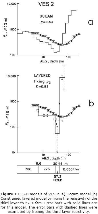
Vertical Electric Sounding. At this site a resistivity sounding (VES 2) parallel to the creek, with origin at x=49 m, was done. Its origin is 54 m from the granitic wall and its spread is approximately parallel to the wall (Figure 9). The data are of good quality (Figure 11), with standard errors of 8%. The curve shape is similar to that of VES 1. With the aim of estimating the subsurface dip of the granitic wall we acquired another resistivity sounding (VES 2b, not shown) whose origin was 25 m from the wall. Unfortunately, these data turned out to be useless because of their high dispersion. This sounding was measured in September, six months after the rain season. High contact resistances in the dry sand surface layer prevented the injection of the current, which were 25 times smaller than those of VES 1 and 2.

Transient Electromagnetic sounding. We acquired nine soundings, eight of them with the off–loop array with 15 by 15 m loops and one in–loop sounding with a 50 by 50 m loop (Figure 9b).

Site 3

VLF–R profiling. The profile is 98 m long with 10 m spacing between readings. At both ends of this line there are barbed–wire fences (Figure 12a); at the southern end, the fence has wooden posts, while at the northern end the posts are metallic. The observed tilt data (Figure 13b) show increasing values as we approach the northern fence, with the Cutler response reaching values close to 50°. In contrast, there are no anomalous values close to the southern fence. There are no anomalous zones in both apparent resistivity profiles (Figure 13c). The plan view of the horizontal magnetic fields shows anomalous values close to the northern fence, especially in the response of the Cutler transmitter (Figure 13d).

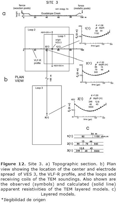
Vertical Electric Sounding. The data of VES 3 (not shown) are highly scattered and shares some of the problems of the VES 2b. It was also measured in September (during the dry season). To reduce the high contact resistances we attempted the use of salty water in the electrodes and increasing the burial depth of the electrodes. We also tried the use of two different equipments, with unsuccessful results.

Transient Electromagnetic sounding. Three in–loop soundings were measured in this site; two of them over the VLF–R line and another 160 m northeast (Figure 12b). The dimensions of loops 1, 2, and 3 were 50 by 50 m, 75 by 75 m y 100 by 50 m, respectively.

 

Numerical methods

2–D modeling of VLF–R data

The VLF–R data were modeled with a 2–D algorithm (Madden and Swift, 1969; Swift, 1971; Vozoff, 1971) that calculates the VLF electromagnetic fields using the analogy that exists between the electromagnetic induction in a 2–D medium with a transmission surface (Swift, 1971). In this method the subsurface and the air layer are divided into an irregular rectangular grid, using smaller cells close to the surface and in the vicinity of resistivity contrasts. For a laterally incident plane wave the problem is solved for two polarizations: the TE mode that involves the E_y, H_x, and H_z fields, and the TM mode, that considers the E_x, E_z, and H_y fields, where the y–axis is the two–dimensionality direction. To account for the different intensities of the primary magnetic fields of the two modes in this code, in a first step all the calculated fields were normalized by the horizontal magnetic field of a "normal" station located far away from the anomalous zone. Then, all the TM mode normalized fields were multiplied by cos(a)and those of the TE mode by sen(a), where ais the angle formed by the total h orizontal magnetic field at the "normal" station with the strike direction. In here we use the measured azimuths of the total horizontal magnetic fields shown in Figures 3, 10, and 13. Finally, to define the tilt angle of the vertical polarization ellipse and the apparent resistivities, we normalize by the intensity of the total horizontal magnetic field, to reproduce the process done by the field equipment.

1–D inversion of resistivity data

The resistivity soundings were inverted to one–dimensional (1–D) models using Occam and layered models. In the former, the model is composed of a large number of thin layers where the resistivity variation between layers is forced to be small, resulting in smooth models. In the latter, the traditional approach to interpret VES data, a small number of layers are used without any imposed restriction on their resistivities.

In the Occam inversion the objective function (U), composed by the data misfit and model roughness terms, is minimized (Constable et al., 1987),

U(ρ) = βx (data misfit) + model roughness

In this expression if the value of βis small, the model is smooth but the data misfit is large. Alternatively, if βis a large value, the misfit error is small but the model is rough.

In the Occam inversion there are several parameters that affect the selection of the final model, such as the first layer thickness, the depth to the deepest interface, the number of layers, and the β parameter. We used the following criteria for these parameters: a) The thickness of the first layer and the depth to the deepest interface were defined as half the shortest and longest electrode spread (AB/2), respectively, based on an often used interpretational guide, that the maximum depth of investigation is half AB/2; b). The number of layers is equal to the number of apparent resistivities; c) A compromise between the misfit error and the model roughness was searched to select the best Occam model.

For the inversion of the data to layered models we used a weighted least squares linearized algorithm based on the singular value decomposition of the derivatives matrix, regularized through the truncation of small singular values (Jupp and Vozoff, 1975). Layered models are very popular in the interpretation of VES. However, the final layered model may reflect more the preconceived ideas of the interpreter than the subsurface information contained in the data, especially when the number of layers is large. Through a smooth variation of ρ(z), Occam tend to respond only to the information contained in the data as they do not depend on the initial model used in the inversion.

In both inversion methods the derivative matrix and the data are weighted by the data errors. For the root mean squared (rms) error we used

where m is the number of data, d_i is the observed apparent resistivity, i = 1,..., m, c_i is the calculated apparent resistivity from the inverted model, and σ_i is the data standard error. A unit value of ε indicates the calculated response fits the observed one as well as the data errors permit. A value less than one indicates overfitting.

To estimate the best layered model we used a Monte Carlo–type (Sambridge and Mosegaard, 2002) searching process. A best–fitting model was first defined, using as initial guess in the iterative inversion, a model based on the behavior of the Occam model. All parameters of the resulting model were randomly perturbed up to +/– 25% of their values in order to define new initial guess models. If one of the inverted models has a misfit error less than that of the current best model, it replaces it as the best model. This process was repeated about 50 times. This procedure tries to find the global minimum in the error hyperspace avoiding the trapping of the solution in a local minimum. With this process we also estimated the parameter uncertainties of the best model. For this, we used the variation ranges of each parameter considering all models that had misfit errors within 5% of the best model misfit.

2.5–D modeling and inversion of resistivity data

Two numerical techniques in two and a half dimensions (2.5–D) were used to model and invert the DC data in this work. The term "two and a half dimensions" is commonly used in geophysics when the 3–D voltage due to a point current source is calculated over a 2–D electrical subsurface.

The algorithm proposed by Dey and Morrison (1979) was used to calculate the voltage V(x, y, z) of several point current sources over an inhomogeneous 2D halfspace, where the resistivity ρ(x, z) does not vary in the y direction. In this me thod the voltage is previously transformed to V(x, k, z) with a Fourier transform in the y direction. The subsurface to be modeled is discretized into an irregular rectangular grid, approximating the resulting Poisson's equation with finite differences for different wave numbers k . The potential V(x, y, z) in the space domain is obtained from the inverse Fourier transformation of the potential in the wave–number domain,

Dey and Morrison (1979) evaluate this integral by dividing the integration interval into sections, approximate the potential in each section with exp(—ak_y) and use the following known integral,

which works well when the y coordinate of the potential electrodes is small or zero.

The approximation (5) to integral (4) was successfully used to model our dipole–dipole profile, where the y coordinates are zero. However, this approximation did not work well for modeling our 1 and 2 VES. In these two cases the electrodes are expanded in a direction parallel to strike, where the y coordinates of the potential electrodes are very different from zero. To circumvent this problem the Fourier transform was evaluated with the convolution method with the filter weights published by Anderson (1975).

In the interpretation of the dipole–dipole profile we also used the 2.5–D approximate inverse solution of Pérez–Flores et al. (2001). Besides discretizing the inhomogeneous subsurface into a rectangular grid, in this technique a compromise between the data misfit and the model roughness is sought through the parameter mentioned above.

1–D Inversion of TEM sounding

The inversion to layered models was carried out with the same least squares linearized technique used for the inversion of the VES. The solution of the TEM forward problem required by the inversion is calculated following the procedure proposed by Newman et al. (1987). The required Hankel and Fourier sine transforms were evaluated by convolution using the weights published by Anderson (1975) and Anderson (1979), respectively. To avoid the time–consuming integration along the loop, each loop side was divided into N wire segments of equal length, approximating each segment by an equivalent electric dipole (Stoyer, 1990). At least three equivalent dipoles for each loop side were considered. The effect of the receiver coil finite bandwidth was incorporated by multiplying the transfer function of the coil by the frequency domain magnetic field. Finally, the effect of the actual current waveform (linear turn–off periodic ramps) was accounted for by using the procedure described by Fitterman and Anderson (1987). This approach requires extrapolating the voltage response beyond the last late–time gate. We fitted a time decaying function to the last five voltages to perform this extrapolation, calculating additional voltages points if necessary. The best fitting layered model was estimated with a Monte Carlo type searching process, in a similar way as done for the VES data. Single or pair of parameters were also perturbed when we expected to have low resolutions or when two parameters were correlated. The process was repeated about 40 times. These results were used to estimate the parameter uncertainties.

2–D simulation of TEM soundings

Unfortunately, we could not model the TEM data in 2.5–D because of lack of the computer code that calculates the response of a 2–D earth excited by a current loop. Nevertheless, to gain insight into several aspects of the fields, we carried out numerical simulations with a modified version of the transmission surface analogy code described above. In this algorithm the subsurface resistivity distribution is 2–D and the source is a pair of 2–D current lines of opposite polarities, such that the electromagnetic fields are purely 2–D.

The fields produced by line current sources are different from those due to a square current loop. This is illustrated in Figure 14, where we compare the voltages induced in a horizontal coil laid over a homogeneous half space of resistivity 300 Ω·m produced by three types of sources: a pair of 2–D current lines of opposite polarity, a square loop, and a vertical magnetic dipole. The separations between the receiver and the sources are similar in the three cases. The currents in the three sources are unit step–off waveforms. The transient voltage produced by the current lines is significantly stronger than that produced by the loop (Figure 14). Furthermore, the voltage from the line sources decays slower with time. For late times, the voltage decays as t^–2 for the line sources and as t^–2.5 for the loop. In the log–log plots such decays translate as straight lines with –2 and –2.5 slopes, respectively. The vertical magnetic dipole (VMD) voltage curve of Figure 14 was calculated with a dipole moment equal to the loop moment (current times area) and the receiving coil 47.5 m from the dipole, that is, replacing the loop by a dipole at its center. An interesting feature of this comparison lies in the resemblance between the VMD and loop voltages. This behavior can be explained by comparing the diffusion depth (δ) with the transmitter–receiver separation (R). The diffusion depth is an estimator of the depth and lateral distance where the current density reaches its maximum value. For this model the ratio R/δ is less than unity at all times for both sources, that is, the transmitter–receiver separation is small with respect to the diffusion depth.

The 2–D numerical simulations were performed to calculate the transient fields in two cases: the underground current density and the voltage induced at a horizontal coil at the surface. For the case of current density, we first calculated the y–component of the electric field at 100 frequencies, from 10^–2 to 10⁸ Hz with the transmission surface analogy code at several points in the subsurface. To transform the frequency–domain electric field to the time–domain we used,

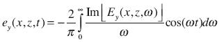
evaluated by convolution with the filter of Anderson (1975). The required current density was finally determined with J(x, z, t) = σ(x, z) e_y (x, z, t). For the case of transient voltages, we used the same code and frequencies, but now to calculate the vertical component of the magnetic field. These fields were transformed to the time–domain voltages with

evaluated again with the filter given by Anderson (1975). Finally, the late–time apparent resistivity was calculated with

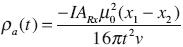
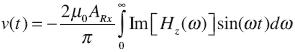
where x₁ and x₂ are the distances that separate the positive and negative sources from the receiver. This expression is obtained from the late–time asymptotic approximation of the voltage from a linear source (Spies and Frischknecht, 1991).

 

Data inversion and modeling

Site 1

VLF–R data. The tilt angle and apparent resistivity responses were modeled in 2–D with a linear conductor immersed in a stratified host (Figure 15a). The metallic pipe was simulated by a 25 by 25 cm conductor of resistivity 0.02 Ω·m located between x= 99.75 and 100 m, with its top at a depth of 1.25 m. The actual pipe diameter is 17 cm. The 2–D grid is formed by 32 and 52 nodes in the vertical and horizontal directions, respectively, with small cell sizes near the surface and near the conductor. The surface responses were calculated at a frequency of 24.4 kHz, the mean value of the two antennae frequencies. For the layered host we used the model obtained from the VES 1 (host A) and the average model obtained from the TEM soundings not perturbed by the pipe (host B). More details on how these 1–D models were estimated can be found below. The fits between the tilt responses (Figure 15b) are good except in the northern shoulder of the Jim Creek tilts, where the calculated response is systematically smaller than the observed data. The fit in this zone could improve if we had included local resistivity variations in the host medium. However, we did not try this as the aim was to keep the models as simple as possible. It is worth mentioning that the skin depth, the depth at which the horizontal magnetic field has decayed to 37% of its value at the surface, is approximately 40 m.

The comparison between apparent resistivity responses is shown in Figure 15c. The effect of the pipe is manifested as a local minimum at x=100 in both antennas. Far from the pipe the calculated apparent resistivities are systematically higher than the observed ones, for both antennas and stratified media, but the difference is more pronounced for host A, the model based on the inversion of the VES 1.

Vertical electric sounding. Figure 4a shows the preferred Occam model for VES 1 and how their calculated response fits the observed apparent resistivity data. This solution is close to the vertex of the misfit versus model roughness curve (Figure 4b), where the condition of a compromise between misfit error and model roughness is satisfied (Hansen, 2000). Occam models are useful as they allow the determination of the main subsurface structure contained in the data (Constable et al., 1987). However, its usefulness decreases in geohydrologic applications as we require discrete depths to the geologic interfaces. This point is illustrated in the model of Figure 4a. The gradual resistivity increase at large depths is undoubtedly due to the presence of the granitic basement, an important geohydrologic parameter. However, it is not possible to define the depth to the resistive substratum as it could be located between 40 m (where the resistivity starts to rise) and 126 m (the deepest interface). The inversion to layered models is a more adequate approach for this task.

Two possible four–layered models for VES 1 are shown in Figure 4c and d. Figure 4c displays the observed apparent resistivities, the unconstrained inverted model, and its calculated response when all the parameters are freed to vary in the inversion. The error bars in the model represent the estimated uncertainties in the parameters. Arrows in the ends of some bars indicate that the estimated range of variation falls outside the plotted area. An important feature of this model is the high uncertainty in the resistivity and thickness of the third layer, result of an equivalence problem in the conductance of this layer. Its resistivity may vary from 3 to 203 Ω·m and its thickness from 1 to 107 m, such that the depth to the underlying resistive halfspace may vary from 16.3 to 122 m. This equivalence problem occurs when a low–resistivity layer is too thin for its depth and too conductive respect the overlying layers, such that its conductance (thickness over resistivity ratio) is well resolved by the data, but not its resistivity and thickness separately. Then, there are many thickness–resistivity pairs with about the same conductance and whose models reproduce the data approximately with the same misfit errors.

The ambiguity associated with this equivalence problem can be reduced by using the lithology information from the nearby well CESPE–1. This well, with a total depth of 63.4 m and located less than 100 m from the VES 1, found altered and fresh granodioritic basement rocks at the depths of 48 and 56 m, respectively. Taking into account that there is a 3.5 m height difference between the location of the resistivity sounding and the well head and that the altered granodiorite po–ssibly has a low resistivity, the depth to the basement under VES 1 was assumed to be 52.5 m (Figure 4d). This depth was included into the layered inversion by constraining the depth to the base of the third layer to be at 52.5 m. The misfit error of this constrained model (Figure 4d) is 1.27, similar to that of the unconstrained model (1.25), with the advantage of a significantly reduced equivalence problem. In February of 2003, three weeks before acquiring VES 1, the depth to the water table was 19.9 m at the CESPE 1 well (Kretzschmar, pers. comm.). Considering the above mentioned height difference, the water table depth under VES 1 is expected at 16.4 m (Figure 4d). The preferred model does not have an interface close to this value, as the depths to the first and second layer bases are at 6.2 and 34 m, respectively.

Dipole–dipole profile. The apparent resistivity pseudosection measured over the aqueduct (Figure 5a) was first inverted and modeled in 2.5–D with the aim of estimating the pipe resistivity with a DC method. Having an estimated resistivity, the second goal was to test if the pipe affects the apparent resistivity measurements of VES 1.

Several inversion attempts with the method of Pérez–Flores et al. (2001) were carried out by varying the model discretization and values of the βsmoothing parameter. Figure 5b show one of these models (β=0.1). The corresponding calculated pseudosection is similar to the observed one, with a low misfit error (ε) of 0.79. In these misfit errors, we assumed all the data errors are 8.9% of a decade, which was estimated from the logarithmic error mean of the 11 repeated measurements mentioned above. The model resistivities are grouped in three logarithmic intervals per decade. The strong resistivity contrast that must exist between the pipe and the sediments is inverted as a wide and thick zone with relatively low resistivities (Figure 5b). The zone with values between 100 and 215 Ω·m is located between x=100 and 101, is 1.5 m wide and 3 m thick. This model does not satisfy our objective of estimating the pipe resistivity. The attempt of rougher models (lower β values) resulted in several zones with strong vertical and horizontal resistivity variations, suggesting that we were fitting the noise, which is significant in these data.

As an alternative approach we opted to model the response by trial and error with the finite differences technique, applying the following constraints: the inhomogeneity representing the pipe has a 0.25 by 0.25 m cross section, it is located between x = 99.75 y 100 and its top is at a depth of 1.25 m. These are the parameters estimated in the 2–D modeling of the VLF–R data. Regarding the host medium, we tried to keep it as homogeneous as possible, including only a general decrease of the resistivity with depth, as this was the 1–D structure found with VES 1. The initial host resistivity distribution was defined from the previous inversion results. The best model and its response are shown in Figure 5c. The visual comparison of the observed pseudosection (Figure 5a) with the calculated one (Figure 5c) gives the impression of a deficient fit. However, the rms misfit error is 1.33, a value comparable to those obtained in the 1–D inversion of the VES. This apparent contradiction is produced by the significant dispersion in the data; the assumed standard error of 8.9% of a decade translates into a linear error of 22%, which is higher than those of the Schlumberger soundings. The estimated pipe resistivity in this model is 0.3 W–m, but may vary from 0.1 to 3 W – m with similar misfit errors.

Once obtained the estimated pipe resistivity, we tested if its presence affects the apparent resistivities of VES 1 using the 2.5–D technique of Dey and Morrison (1979). In the actual field conditions (Figure 2) the sounding center is 60 m from the pipe with the electrode array expanding in the direction parallel to the pipe. At this distance the pipe does not affect the sounding data; it starts to produce a significant perturbation only when the sounding is at a distance of about 10 m. Figure 16 displays the perturbed responses calculated when the pipe is 5 and 10 m from the electrode array, comparing them with the apparent resistivities of the unperturbed four–layered model of Figure 4d. The pipe produces a local minimum–maximum pair which grows in magnitude and moves toward the short electrode separations as the distance to the pipe decreases.

Transient Electromagnetic Soundings. Most of the TEM were inverted to layered models. To illustrate the general behavior of the models, Figure 6 shows the results for loop 4, which is the loop with the most complete sequence of receivers. We include the observed apparent resistivity data as a function of time of 10 soundings, the layer resistivities and depths of 8 inverted soundings, together with their calculated responses and misfit errors. All these models are of three layers. The misfit errors are adequate, with values varying from 0.69 to 1.48. The general behavior of these models is of a resistive–conductive–resistive sequence, interpreted as the vadose zone–aquifer–resistive basement sequence. We could not find any model for soundings 4(3) and 4(2). For them the receiver coil was located within 5 m of the pipe location inferred from the VLF–R data. The perturbing effect of the pipe is so intense in these receivers that the data could not be fitted to any layered model.

In the numerical simulation to be presented below we show that the lateral effect of the pipe can be neglected if both the transmitter and receiver are located more than 60 m from the pipe. Figure 7a shows the data and calculated responses of six soundings that fulfill this condition, while Figure 7b displays the corresponding models. Despite reasonable fits (the rms errors vary from 0.80 to 1.49) and obtaining the same three–layered sequence (resistive–conductive–resistive), there is an important parameter variability in these models. For example, the depth to the top of the conductor varies from 8.4 m to 24.9 m and its resistivity from 37 to 101 Ωm. It is unlikely that the actual resistivity structure has these variations in such a short distance. Such variability is probably due to noise in the data.

By logarithmically averaging the layer parameters of the six models we estimate an average model (Figure 7b). The average and standard deviations of the resistivities are: 3,400 +/– 2,200, 70.2 +/– 27.7 , and 36,000 +/– 20,000 Ωm. For the depths we have: 16.2 +/– 7.6 and 44.3 +/– 7.6 m. This average model shows a good agreement with the nearby CESPE–1 well (Figure 7b). The water table measured in March 2003 was at a depth of 16.4 m, while the average TEM depth to the conductor is 16.2 m. The depths to the altered and unaltered granodiorite are at 44.5 and 52.5 m, respectively (Figure 7b), while the average TEM depth to the resistive substratum is 44.3 m.

Figure 8 shows a sensitivity analysis of the TEM model of sounding 1(4). The comparison between observed voltages and apparent resistivities with the corresponding model responses are included in Figure 8a and b. The inverted resistivity model as a function of depth and the estimated parameter uncertainties are shown in Figure 8c. The uncertainties of the first and third layers are very large (an arrow at the end of the error bar indicates that the uncertainty falls beyond the plotting area), while those of the second layer resistivity and the depths to its top and base are relatively small. These features are confirmed by analyzing the elements of the sensitivity matrix or derivatives of the data respect to the model parameters. In Figure 8d we plot the derivatives as a function of time, also known as sensitivities, where v_i is the i'th calculated voltage, p_j is any of the five model parameter, and σ_i, is the i'th voltage error. The low resolutions of the first and third layer resistivities are due to very low derivatives with respect to ρ₁and ρ₃ , that is, the data contain little information on these parameters. Although hardly seen in Figure 8d, the highest values of the p_l derivative are those of the shortest times. If we would have been able to measure the voltages at times much shorter than 6.8 ps, which is the earliest time for the TEM47 system, we would have a better resolution for this resistivity. In contrast, the errors of the top, base, and resistivity of the second layer (Figure 8c) are small because the corresponding derivatives are significantly greater. It is important to notice that this layer does not have an equivalence problem like that affecting the model of VES 1. In the presence of a thin conducting layer the electromagnetic methods are less affected by equivalence than the DC galvanic methods (Fitterman et al., 1988).

The results of a 2–D numerical simulation for loop 4 are shown in Figure 17. The model is composed of a linear conductor (simulating the pipe) embedded in the first layer of a three–layered host medium (Figure 17a). A pair of linear current sources of opposite polarity, located at x=–15 and 15 m, energize the subsurface. The conductor has a 25 by 25 cm cross section, its top is at a depth of 1.25 m, and has a 0.02 Ωm resistivity. The host medium is the average undisturbed TEM model depicted in Figure 7b. The distances between source and inhomogeneity simulate the field geometry of loop 4. The magnitudes of the current density perpendicular to the section are shown at 7 and 35 ps after the unit current is turned off (Figure 17b). The first time (7 μs) is approximately equal to the shortest time (6.8 μs) of the TEM 47 system. The current density contours are plotted only in the quadrant 0 < x < 150 m, 0 < z < 150m; if the inhomogeneity is excluded, the current density has odd symmetry respect to the plane x=0.

Several interesting features can be drawn from Figure 17b:

a) The global maxima occur at the conductive inhomogeneity representing the pipe. Because of its low resistivity, strong currents are induced in it, which are more than three orders of magnitude greater than the local maxima located in the host medium.

b) The local maximum at 7 ps attenuates and laterally migrates with time in a similar behavior to the "smoke rings" of Nabighian (1979), where the current density decreases and the ring radius increases with time. At 7 μs the maximum is at the coordinates (x=42.5, z=25 m) and has an intensity of 33x10^–6 A/m². At 35 μs the maximum is wider, has migrated in depth and to the right to (113,30) and its intensity has decreased to 3.5x10^–6 A/m².

c) The local current density maximum is trapped by the layer of lower resistivity. In a homogeneous 300 Ωm model, the maximum at 35 μs is at a depth of 60 m; in our model it is at 30 m depth. This is explained by the preference of the current to flow in the medium of less resistance, that is, the 70.2 Ωm layer.

d) At 7 μs a large part of the total current is already flowing in the conductive layer while only a small portion is flowing in the shallow, first layer. This explains the low resolution of the TEM data to the resistivity of the first layer.

To evaluate how far the pipe affects the TEM measurements of loop 4, Figure 18 shows the apparent resistivity responses of the stratified model without pipe (model A) and with pipe (model B), at three sites located at different distances from the source (x=–22.5, 15, and 45 m). The x origin is again located between the two line sources. We considered a horizontal coil of unit area as the receiver. The three responses from model A are different because of the variable transmitter–receiver separations, but they clearly show the presence of a low associated with the conductive layer. On the other hand, in the responses from model B the pipe effect is very intense at the receiver located at x=45, decreases at x=15 and is almost null at x=–22.5 m. This latter receiver simulates the position of sounding 4(10) from loop 4, which is about 70 m from the pipe. These results suggest that the actual data of sounding 4(10) could be safely interpreted with a 1–D model. As the electric field at the pipe impressed by a pair of line current sources is more intense than that impressed by a square loop, the 70 m separation can be considered as the upper limit of the perturbation distance, such that, for the actual square loops, this distance could be reduced to about 60 m. It is important to point out that we can not directly compare these responses with the actual data of site 1 because of the differences illustrated in Figure 14.

Site 2

VLF–R data. Figure 19 displays the VLF–R modeling results. The 2–D model consists of a stratified medium laterally interrupted by a resistive contact with a 60^o dip (Figure 19a). The topographic effect of the granitic wall is also included in the model by considering a hill with a height of 50 m and 45^o slope. The layered structure is that obtained from the 2.5–D modeling of VES 2. As the measured profile is 33^o off from the normal to the wall, the 2–D results are projected into the profile. The fit in the tilt response from Cutler (Figure 19b) is not optimum. However, the low observed intensities are well reproduced. The strong tilt anomaly from the Jim Creek antennae is well fitted by the calculated response (Figure 19b). In contrast, the calculated apparent resistivities are systematically greater than the measured ones (Figure 19c). At the right end of the profile, where the effect of the resistive block is negligible, the calculated apparent resistivities are approximately 300 Ω·m, while the observed ones are about 50 Ω·m. As the stratified medium is based on the interpretation of VES 2, this discrepancy suggests a significant disagreement between the VLF–R apparent resistivities and those of the Schlumberger sounding, in a similar way to that in site 1.

Vertical Electric Sounding. The preferred Occam and layered models of VES 2 are shown in Figure 11. The fits between calculated and observed responses are good, with misfit errors of 0.53 and 0.52, respectively. We were forced to consider misfit errors less than unity, indicating data overfitting. For errors close to unity the misfits were large for large electrode spreads. In a first try the data were inverted to unconstrained four–layered models, i.e., with all layer parameters varying during the inversion process. All these models share a strong equivalence problem in the conductance of the third layer. This obviously produces a large uncertainty in the depth to the basement. To circumvent this problem, we constrained the inversion (Figure 11b) by fixing the third layer resistivity in 57.3 Ω·m, which is the inferred value of the corresponding layer in the constrained inversion of VES 1. With this approach the depth to the resistive basement is 43.7 m. In the layered model of Figure 11b we include two types of parameter error bars; those with a solid line are estimated with the resistivity of the third layer fixed, while those plotted with dashed lines were estimated by considering this resistivity free to vary. For the latter, the largest error bars correspond to the conductive layer, confirming the equivalence problem. Constraining this resistivity clearly reduces the equivalence, notably decreasing the uncertainty in the conductor thickness.

The granitic mass outcropping in the southern end of this site may affect the apparent resistivity measurements of the VES 2. To evaluate this possibility we used the finite differences. Figure 20 shows the 2.5–D modeling results. The center of the Schlumberger sounding is 53 m from the granitic wall and the electrode spread is parallel to it. Using the modeling result of the VLF–R data, the granitic block was also simulated with a 60^o dipping fault contact (Figure 20a), while for the layered structure of the sediments, we initially considered the four–layer model of Figure 11b. The final model, obtained by trial and error, is shown in Figure 20a. The measured apparent resistivities of VES 2 and that calculated from the model are shown in Figure 20b. The fit is satisfactory, with an rms error of 0.78. In relation to the initial model, we had to modify the basement depth and resistivity under the sounding and the resistivity of the conductive layer. Certainly, it would have been desirable to have more VES sounding to better constrain the dip of the resistive block. As mentioned above, we attempted to measure one more sounding closer to the wall, but high contact resistances prevented the acquisition of good data.

Transient Electromagnetic Soundings. The TEM soundings of this site were inverted to three–layered models, all of them with a resistive–conductive–resistive sequence. The results are depicted in Figure 21, where we include only the models of loops 2 and 3. The misfit errors are slightly greater than those of site 1, varying from 1.13 to 1.64. An important feature of these models is that the conductive layer has a very low resistivity (about 12 Ωm), is shallow (from 5 to 19 m), and very thin (2 to 3 m thickness), such that the resistive substratum is found at depths from 7 to 22 m. These depths are much smaller than the 73 m estimated with the 2.5–D modeling of VES 2. Such strong discrepancy might be caused by the lateral effect of the granitic block. We carried out a 2–D simulation to explore this possibility. The model (Figure 22a) is the same to that obtained for VES 2 with 2.5–D modeling, consisting of a stratified medium laterally bounded by a 60^o dipping fault. The pair of current lines are 15 m apart, simulating loop 2. The voltage and apparent resistivity responses were calculated at x=–37.5 and 37.5 m, reproducing the receiver positions of soundings 2(4) and 2(1), respectively. The comparison of apparent resistivity responses between the layered model and the one that includes the lateral contact is shown in Figure 22b. The lateral effect of the resistive body manifests as a superimposed maximum in the curve denoted as "layers + fault", producing the formation of two relative minima. In the sounding closer to the fault (x=–37.5) this maximum occurs at shorter times than in the farther sounding (x=37.5). To compare these results with the actual data, Figure 22b includes the observed apparent resistivities of soundings 2(1) and 2(4), where these responses only cover the times from 7 μs to 70 or 100 μs. If we invert the synthetic data of the farthest receiver (x=37.5) to a layered model we would obtain a shallower and thinner conductor and, consequently, a resistive substratum at a shallower depth than the true depth. This behavior is similar to the

1– D models of the actual data (Figure 21). However, the observed data at sounding 2(4) still shows a pronounced minimum, differing from the behavior of the corresponding synthetic response. This discrepancy suggests that this

2– D model is not adequate. It is possible that the geometry of the fault contact is more irregular than a simple dipping plane. Other possibilities are 3–D effects due to the non–orthogonality of the line respect to the wall (57°) or associated with the change of strike of the wall several tens of meters away from the site.

Site 3

VLF–R data. The intense tilt anomalies occurring at the northern end of the VLF–R profile, associated with the fence with metallic posts, was modeled in 2–D with a 0.004 Ω·m vertical conductor 1.5 m high and 2 cm wide (Figure 23a). For the host medium we used the three–layered model estimated from the TEM sounding 2(1), to be described below. Here we did not used as host the model derived from the Schlumberger sounding because of the low quality of these data. The fits between the calculated and observed tilt responses are good (Figure 23b), as the peaks and decaying rates from both antennae are well reproduced. The tilt anomaly from Cutler is more intense than that from Jim Creek because the horizontal magnetic field is practically normal to the fence (see Figure 13d), producing a close–to–maximum electromagnetic coupling in the TE mode, the one associated with the anomalous vertical magnetic field.

Regarding the apparent resistivities (Figure 23c), the calculated response for Cutler shows a slight decrease close to the fence, but the data dispersion is greater than the anomalous response, such that little can be inferred from the apparent resistivities. However, notice that the calculated responses do follow the general trend of the observed data, contrasting to what happened at sites 1 and 2. A further analysis of these points will be dealt in the discussion section.

We also calculated the VLF–R responses of the fence with wooden posts by simulating the three barbed wires with three conductors of 2 by 2 mm cross sections, at 0.5, 1, and 1.5 heights, all with 0.004 Ω·m resistivities, using the same host medium of Figure 23. The tilt response at x=0, 3 m away from the fence, is less than one hundred of a degree, confirming then the absence of any tilt anomaly in the southern end of the profile.

Vertical Electric Sounding. The misfit errors of the Occam and layered models of VES 3 (not shown) are high (3.03 and 2.19, respectively), mainly due to high dispersion in the data and large misfits for large spreads. The three–layered inverted model has a resistive–conductive–resistive sequence. The second layer tentatively could be assigned to the aquifer, with a depth of 2.7 m to its top. However, this depth has a poor correlation with the information from nearby wells, where the watertable is found at a depth of 26 m in a well 1.5 km to the east and at 10 m in other well 500 m to the west, such that a depth between these two values is expected under the resistivity sounding. The low quality data and a too shallow conductor lead us to conclude that the apparent resistivity data are contaminated by noise that severely hinders its interpretation. The culprit should be the high contact resistances that limited the injected currents, producing then noisy voltage measurements. This sounding was acquired six months after the end of the rain season. Loss of the water content in the surface sands is the likely source of the high contact resistances.

Transient Electromagnetic Soundings. The models of the three in–loop soundings are shown in Figure 12c. They are of two and three layers, with good misfit errors varying from 1.0 to 1.1. The model of sounding 1(1) is similar to that of sounding 2(1), which has a weak resistivity contrast between their first and second layers. The three–layered models are again interpreted as the sequence unsaturated zone–aquifer–granitic basement. The mean values of the resistivity of the conductive layer and their depths to its top and base are 68 Ω·m, 13.7 m and 49 m, respectively. Unfortunately, the low quality of VES 3 and the absence of a close–by well preclude the confirmation of this interpretation. The only other piece of nearby information comes from the Schlumberger sounding 208 measured by Díaz–Curiel (1986), located 100 m from site 3. The interpretation of this sounding gives a 30 m depth to the resistive substratum, such that there is an important discrepancy with the mean depth of 49 m estimated with the TEM soundings.

In this zone there are no obvious geologic inhomogeneities that might affect the 1–D interpretation of these soundings, but the presence of the fence with metallic posts could represent an important source of noise. In the VLF–R method this fence produced the strongest tilt angle anomaly of the whole study. In the 2–D modeling of these data we estimated a fence resistivity of 0.004 Ω·m. To estimate the effect of the fence in the TEM data we carried out a purely 2–D numerical simulation. The model (Figure 24a) consists of a three–layered earth with a highly conductive strip at the surface representing the fence. The layered model is that obtained by inverting sounding 2(1). The locations of the pair of current lines and of the receiving coil also simulate this sounding. The positive line current is 22.5 m from the fence. The comparison between the calculated responses without (solid line) and with fence (circles) is shown in Figure 24b. The conductor does affect the apparent resistivities, producing a minimum slightly more intense than the response without fence. If we invert the response with fence, the depth to the resistive substratum would be greater than the true depth. This effect explains the discrepancy between the 49 m depth estimated with the TEM soundings and the 30 m estimated with VES 208.

 

Discussion

Because of the large variety of geophysical methods, sites, survey parameters, and modeling techniques used in this work, it is convenient to present first a summary of the results obtained for each type of inhomogeneity, to proceed with other points that deserve a separate discussion.

The pipe. The presence of the metallic pipe was clearly detected by the tilt angle measurements in the VLF–R method. With a 2–D model of these data, we estimated a pipe resistivity of 0.02 Ωm. As layered hosts we considered the model from VES 1 and an average TEM model not perturbed by the pipe. The tilt angle fits are satisfactory in both cases. The cover that protects the pipe is not good enough to insulate it from the current impressed with the dipole–dipole array. Even with a pipe resistivity of about 0.3 Ωm, the nearby Schlumberger sounding is not affected by the metallic pipe. Most of the TEM soundings are perturbed by the presence of the pipe. With a 2–D numerical simulation we estimated that its lateral effect is negligible when the loop and receiver are more than 60 m from the pipe.

The granitic wall. The presence of this resistive block affected the response of the three geophysical methods. The VLF–R data were modeled using a 2–D contact with a 60^o dip plus a stratified ground inferred from the VES 2. Reasonable fits resulted for the tilt angles of both antennae.

The fence with metallic posts. This object, located near the end of the VLF–R profile in site 3, produced the strongest tilt anomaly of all the study. However, fences with wooden posts located in sites 1 and 3 did not give any anomalous response. Why the metallic–post fence produces such a strong anomaly in the VLF–R tilt data and not the wooden–post fences? There are two physical mechanisms that can explain these findings. The metallic posts allow the induced current in the horizontal wires to be closed between each pair of vertical posts, producing vertical cells of current that are more efficient in producing anomalous magnetic fields than the simple induction in the wires. Another mechanism is the leakage of current into the ground via the metallic posts. Although the simulation of vertical cells of current is not possible with the 2–D algorithm used to model the data, we estimated an equivalent resistivity (0.004 Wm) for the metallic post fence.

Stratified media. In site 1 the layered model of VES 1 suffers from a strong equivalence problem. We used a priori information (the depth to the granitic basement in a close–by well) to constrain this model. In the resulting model the depth to the conductive layer does not agree with the measured water table depth. Although there are other models that do agree, they are not of minimum misfit error. The layered inversion of six TEM soundings located more than 60 m from the pipe gave similar resistive–conductive–resistive structures, but with an important variability in the model parameters, likely due to noise in the data. However, the average model shows reasonable agreements with the depths to the water table and basement encountered in the nearby well. The resistivities of the resistive layers have low resolutions, but not the depths and resistivity of the conductive layer, such that they are not affected by the equivalence problem hindering the VES 1.

In site 2, the VES 2 layered model is also affected by an intense equivalence problem that limits the accurate estimation of the depth to the resistive substratum. To constrain the 1–D inversion we fixed the resistivity of the conductive layer to the corresponding value found for VES

1. The VES 2 sounding data are perturbed by the presence of the resistive block, modelled with a 60^o dipping fault. The layered inversion of the TEM data systematically rendered models that do not agree with the estimated from VES

2. The 2–D numerical simulation suggests that all the TEM soundings are affected by the lateral effect of the resistive block, invalidating then the TEM layered models. In this simulation the behavior of the synthetic data is similar to the actual response in a receiver located far from the contact, but is different in a receiver close to the contact. This suggests that the model should be more complicated than the proposed one. Possibly the contact is not elongated enough as the wall changes its strike 50 m to the north of the profile. Other possibilities include a change in the fault dip at depth or the presence of large granitic boulders buried in the sediments. These suggest that a 3–D model might be needed to reproduce the data, a task beyond the objectives of this work.

In site 3 the three in–loop TEM soundings rendered similar layered models, with a mean depth to the resistive substratum of 49 m. With a 2–D simulation of one of these soundings we estimated that the fence produces a slightly more intense minimum in the apparent resistivities than that without the fence. This effect could explain the greater depth to the basement (49 m) of the TEM models compared to the 30 m estimated from the nearby VES 208.

Geophysical performance of the VES and TEM methods. In this study both methods showed advantages and disadvantages. The data quality in the VES was variable; in sounding 1 and 2 was good, but bad in soundings 2b and 3. The first two soundings were acquired just after the end of the rain season, while the last two were measured six months later, during the dry season. The presence of high electrical resistance in the dry sand close to the electrodes, known as contact resistance, explains the low data quality in the last two soundings. In them the injected currents were less (by a factor of 20 or 30 with) respect to those injected in the first two soundings, explaining the low signal to noise ratios in the measured voltages. On the other hand, the quality of the TEM data was not optimum but the relative data dispersion was slightly higher than those of VES 1 and 2. High contact resistances are not a limitation of the TEM method as the subsurface currents are created by induction, without the need to inject current to the ground.

Regarding the question of how much the lateral inhomogeneities affect the measurements of these methods, they can be classified as conductive or resistive. The pipe and the metallic–posts fence are conductive inhomogeneities. They affected the TEM soundings in sites 1 and 3. The VES 1 was not perturbed by the pipe, and possibly, neither the VES 3 by the fence. From these results we can generalize that conductive inhomogeneities significantly affect more the TEM soundings than the Schlumberger data. The granitic block of site 2, clearly a resistive inhomogeneity, affected both the VES and TEM measurements.

The shallow structure estimated from the VES is usually well resolved, being the opposite for the TEM soundings. In the latter the first resistive layer was detectable, but its resistivity was poorly resolved by the data, unless the layer had a moderate resistivity value, as was the case for the models of site 3. With the 2–D numerical simulation, we found that at the shortest times the induced currents were already flowing in the conductive layer associated with the aquifer. To improve the shallow resolution it would be necessary to use other equipment with shorter times.

Regarding the deep structure, VES 1 and 2 (and at least four soundings of Díaz–Curiel, 1986), are strongly affected by an equivalence problem in the conductive layer. In contrast, in the TEM layered models not perturbed by the pipe and those of site 3, the equivalence problem is practically absent.

Discrepancy between the calculated and observed VLF–R apparent resistivities. Even when the VLF–R apparent resistivity data are more scattered than those of the tilt angle, it was possible to define clear trends of the former response. However, obtaining reasonable fits between the calculated and observed apparent resistivity responses turned out to be a more difficult task. When the stratified host model was based on a VES, the calculated apparent resistivity response was systematically higher than the observed data. In contrast, when the host model was based on the TEM data, the calculated response showed a fair agreement with the observed response. Pseudoanisotropy (Maillet, 1947; Orellana, 1972) could explain this apparently odd behavior. This physical mechanism occurs when in a set of layers there is an alternation of thin layers of different resistivity, such that the set behaves electrically as a single anisotropic layer, even when every layer in the set is isotropic. This phenomenon is described by the equivalent longitudinal p_L and transverse p_T resistivities, given by,

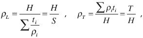
where H, S and T are the total thickness, the longitudinal conductance, and the transverse resistance, respectively, of the set of layers, and p. and t. are the resistivity and thickness of each layer. In these cases the transverse resistivity is always greater than the longitudinal resistance. In the VES method the subsurface current flow in a stratified medium has mostly vertical and horizontal components, then responding to the average resistivity . In contrast, in the VLF–R and TEM methods the subsurface current flow is horizontal, with no vertical component, such that the apparent resistivities derived from these methods depends only on ρ_L. The fact that ρ_m > ρ_L could explain why the VES–based calculated apparent resistivity is greater than the observed response and the closer agreement when the calculated response is based on a TEM sounding. The ratio of 1.7 between the calculated and observed apparent resistivities in site 1 could be explained by the presence of 10 cm thick clay layers spaced every meter in the first 40 m of the resistivity section. The presence of such clay layers, with a nominal resistivity of 20 Ωm, could originate from flooding episodes in the past, which could have been easily missed by the 2 m sampling of surface cuttings at the CESPE–1 well. Therefore, macroanisotropy could explain the discrepancy in site 1. However, it is more difficult to justify it in site 2, where the ratio is at least 3.1

 

Conclusions

With the use of several numerical algorithms, such as 1–D inversion (VES and TEM) and forward modeling in 2–D (VLF–R and TEM) and in 2.5–D (VES), it was possible to estimate the subsurface resistivity structure in some cases, and in others, estimate the distorting effect of the shallow lateral inhomogeneities. Only for the TEM soundings close to the granite wall the need for 3–D methods of interpretation was evident. The application of the VLF–R method in this area was very useful. The anomalies detected with this method indicated the presence of inhomogeneities that could had passed unnoticed by the other methods, affecting the interpretation of their data.

The VES and TEM soundings resulted complementary in several aspects. High contact resistances seriously affected some VES, but not the TEM soundings. Conductive inhomogeneities affected some of the TEM measurements but did not affect the VES data. The shallow resistitvity structure is better resolved with the VES method. The equivalence problem in the conductive layer affected the VES but not the TEM data.

The pipe protective cover is not efficient enough as to insulate it from the galvanic current flow. We estimated a pipe resistivity between 0.1 and 3 Ωm, a value greater than the resistivity inferred from the current induced electromagnetically. Nevertheless, the VES 1 was sufficiently far from the pipe as to be affected by it.

When performing TEM soundings, it is advisable to locate them far from fences with metallic posts as they represent a source of distortion. Fences with wooden posts apparently do not pose any problem. We propose site 1 as a test site for new geophysical methods as the amount of geohydrologic, geologic, and geophysical information and its easy access are benefits not easy to find.

 

Acknowledgements

We are grateful to Jaime Calderón and Alejandro Díaz for their useful assistance in the numerous field trips. We thank Marco Pérez for permitting the use of his inversion algorithm.

 

Bibliography

Anderson W.L., 1975, Improved digital filters for evaluating Fourier and Hankel transform integrals, U.S. Geologic Survey Report GD–75–012.         [ Links ]

Anderson W.L., 1979, Numerical integration of related Hankel transforms of order 0 and 1 by adaptive digital filtering, Geophysics, 44, 1,287–1,305.         [ Links ]

Andrade M., 1997, Actualización geohidrológica del Valle de Guadalupe, Municipio de Ensenada, Baja California. Agosto de 1997. Technical Report to Grupo Agroindustrial del Valle de Guadalupe, 60 p.         [ Links ]

Antonio–Carpio R., Arroyo–Acosta A., Romo–Jones J.M., Vázquez–González R., 2007, Groundwater exploration in Baja California, Mexico, using audiomagnetotellurics, Abstract, American Geophysical Union Fall Meeting, San Francisco.         [ Links ]

Beltrán L., 1998, Actualización hidrogeológica del acuífero del Valle de Guadalupe, Municipio de Ensenada, Baja California, Technical Report, Comisión Nacional del Agua, 24 p.         [ Links ]

Campos–Gaytán J.R., 2008, Simulación del flujo de agua subterránea en el acuífero del Valle de Guadalupe, Baja California, México, Ph.D. Thesis, CICESE, 220 p.         [ Links ]

Constable S.C., Parker R.L., Constable C.G., 1987, Occam's inversion: A practical algorithm for generating smooth models from electromagnetic sounding data, Geophysics, 52, 289–300.         [ Links ]

Dey A. and Morrison H.F., 1979, Resistivity modelling for arbitrarily shaped two–dimensional structures, Geophysical Prospecting, 27, 106–136.         [ Links ]

Díaz–Curiel R.S., 1986, Estudio geohidrológico del Valle de Guadalupe y Valle de Santa Rosa, B.C., Technical Report, Geofísica del Noreste, 85 p.         [ Links ]

Fitterman D.V., Anderson W.L., 1987, Effect of transmitter turn–off time on transient soundings, Geoexploration, 24, 131–146.         [ Links ]

Fitterman D.V., Meekes J.A.C., Ritsema I.L., 1988, Equivalence behavior of three electrical sounding methods as applied to hydrogeo–logical problems, 50th Meeting European Association of Exploration Geophysicists.         [ Links ]

Hansen P.C., 2000, The L–curve and its use in the numerical treatment of inverse problems, in Computacional Inverse Problems in Electrocardiology, P. Johnston (ed.), 119–142, Advances in Computational Bioengineering, vol. 4, WIT Press.         [ Links ]

Jupp D.L.B., Vozoff K., 1975, Stable iterative methods for the inversion of geophysical data, Geophys. J. R. astr. Soc., 42, 957–976.         [ Links ]

Keller G.V., Frischknecht F.C., 1966, Electrical methods in geophysical prospecting, Perga–mon Press, 523 p.         [ Links ]

Kirsch R., 2006, Grounwater geophysics, a tool for Hydrogeology, Springer, 495 p.         [ Links ]

López–Moya A., 2009, Caracterización eléctrica del lecho del Arroyo Guadalupe, Baja California, M.Sc. Thesis, CICESE, 175 p.         [ Links ]

Madden T.R., Swift C.M., 1969, Magnetotelluric studies of the electrical conductivity structure of the crust and upper mantle, in: Penbroke (ed.), The Earth's Crust and upper Mantle, Geophysical Monograph 13, Amer. Geophys. Union, 469–479.         [ Links ]

Maillet R., 1947, The fundamental equations of electrical prospecting, Geophysics, 12, 529–556.         [ Links ]

McNeill J.D., 1990, Use of electromagnetic methods for groundwater studies, in: Ward, S.H. (ed.), Geotechnical and environmental geophysics, Vol. I: Reviews and tutorial, 191–218, Soc. of Explor. Geophys., Tulsa, Oklahoma.         [ Links ]

McNeill J.D., Labson V.F., 1991, Geological mapping using VLF radio fields, in: Electromagnetic Methods in Applied Geophysics, Applications, Part B, by M.N. Nabighian (ed.), 521–640, Soc. of Explor. Geophys.         [ Links ]

Nabighian M.N., 1979, Quasi–static transient response of a conducting half–space: An approximate representation, Geophysics, 44, 1,700–1,705.         [ Links ]

Nabighian M.N., MacNae J.C., 1991, Time domain electromagnetic prospecting methods, in Nabighian, M.N. (ed.), Electromagnetic methods in Applied Geophysics, vol. 2, Applications, Part A, 427–479, Soc. of Expl. Geophys.         [ Links ]

Newman G.A., Anderson W.L., Hohmann G.W., 1987, Interpretation of transient electromagnetic soundings over three–dimensional structures for the central–loop configuration, Geophys. J. Roy. astr. Soc, 89, 889–914.         [ Links ]

Orellana E., 1972, Prospección geoeléctrica en corriente continua, Paraninfo, 523 p.         [ Links ]

Pérez–Flores M.A., Méndez–Delgado S., Gómez–Treviño E., 2001, Imaging low–frequency and dc electromagnetic fields using a simple linear approximation, Geophysics, 66, 1,067–1,081.         [ Links ]

Sambridge M., Mosegaard K., 2002, Monte Carlo methods in geophysical inverse problems, Reviews of Geophysics, 40(3),1–29.         [ Links ]

Spies B.R., Frischknecht F.C., 1991, Electromagnetic sounding, in: Electromagnetic Methods in Applied Geophysics, Vol. 2, Applications, Part A, by Nabighian, M.N., (ed.), 285–386.         [ Links ]

Stoyer C.H., 1990, Efficient computation of transient sounding curves for wire segments of finite length using an equivalent dipole approximation, Geophysical Prospecting, 38, 87–100.         [ Links ]

Swift C.M., 1971, Theoretical magnetotelluric and Turam response from two–dimensional inhomogeneities, Geophysics, 36, 38–52.         [ Links ]

Vozoff K., 1971, The effect of overburden on vertical component anomalies in the AFMAG and VLF exploration: A computer model study, Geophysics, 36, 53–57.         [ Links ]

Ward S.H.,1990, Resistivity and induced polarization methods, in: Ward, S.H. (ed.), Geotechnical and environmental geophysics, Vol. I: Reviews and tutorial, 147–189, Soc. of Explor. Geophys., Tulsa, Oklahoma.         [ Links ]