


Servicios Personalizados
Revista
Articulo
 Inglés (pdf)
 Artículo en XML
 Referencias del artículo
 Enviar artículo por email
Indicadores
-
 Citado por SciELO
 -
 Accesos
Links relacionados
-
 Similares en
SciELO
Similares en
SciELO
Compartir

 Permalink
Geofísica internacional
versión On-line ISSN 2954-436Xversión impresa ISSN 0016-7169
Geofís. Intl vol.50 no.1 Ciudad de México ene./mar. 2011
Original paper
Unified formulation of enhanced oil–recovery methods
Ismael Herrera and Graciela S. Herrera*
Instituto de Geofísica Universidad Nacional Autónoma de México Ciudad Universitaria Del. Coyoacán 04510 Mexico D.F. e–mail: iherrera@geofisica.unam.mx* Corresponding author: ghz@geofisica.unam.mx
Received: June 7,2010
Accepted: October 6, 2010
Published on line: December 17, 2010
Resumen
En la actualidad las técnicas de recuperación mejorada de petróleo (EOR, por sus siglas en inglés) son esenciales para mantener los suministros de petróleo del mundo. A su vez, los modelos matemáticos y computacionales de los métodos EOR son fundamentales para su aplicación y perfeccionamiento. Debido a la gran diversidad de procesos que ocurren en la EOR, es valioso contar con procedimientos generales unificados para la construcción de los mismos, que puedan aplicarse fácilmente independientemente de la complejidad del sistema considerado. El objetivo de este trabajo es presentar un modelo matemático unificado, que incluya ambos: el sistema gobernante de las ecuaciones en derivadas parciales y las condiciones de choque. Éste se basa en una formulación axiomática, pues las formulaciones axiomáticas son el medio más eficaz para lograr generalidad, sencillez y claridad. En el enfoque que se propone aquí, la construcción del modelo matemático es en gran medida automática, todo lo que se requiere a fin de definir las ecuaciones en derivadas parciales y las condiciones de choque que constituyen un modelo básico consiste en identificar las fases y las propiedades extensivas que participan en el sistema de la EOR. Este modelo básico proporciona una base muy firme para incorporar la fenomenología. El procedimiento se ilustra derivando los modelos matemáticos más utilizados en la tecnología EOR; en particular, se derivan los modelos de petróleo negro y los composicionales, tanto en su versión isotérmica como sus variantes térmicas, en las cuales es indispensable incluir el balance de energía. Para ilustrar la aplicación de la formulación axiomática a modelos con discontinuidades, se realiza también una descripción exhaustiva de los choques que pueden ocurrir en el Modelo de Petróleo Negro.
Palabras clave: EOR, recuperación mejorada, modelación matemática, modelo del petróleo negro, modelo composicional, procesos térmicos.
Abstract
At present enhanced oil recovery (EOR) techniques are essential for maintaining the oil supplies of the world. In turn, mathematical and computational models of the processes that occur in EOR are fundamental for the application and advancement of such methods. Due to the great diversity of processes occurring in EOR, it is valuable to possess unified general procedures for constructing them, which can be easily applied independently of the complexity of the system considered. The leitmotiv of this paper is to present a unified mathematical model, including both: the governing system of partial differential equations and shock conditions. It is based on an axiomatic formulation, since axiomatic formulations are the most effective means for achieving generality, simplicity and clarity. In the approach here proposed, the construction of the mathematical model is to a large extent automatic; all what is required in order to define the partial differential equations and the shock conditions that constitute such a basic model is to identify the phases and extensive properties that participate in the EOR system. Such a basic model supplies a very firm basis on which the phenomenology is incorporated. The procedure is illustrated by deriving the mathematical models of the most commonly occurring EOR models: black–oil, compositional and non–isothermal compositional. An exhaustive description of the shocks that may occur in black–oil models is also included.
Key words: enhanced oil recovery, mathematical models, black–oil model, compositional model, non–isothermal compositional model.
Introduction
Generally, three stages of oil recovery are identified in the production life of a petroleum reservoir: primary, secondary and tertiary recovery (Lake, 1989). Primary recovery refers to the production that is obtained using the energy inherent in the reservoir due to gas under pressure or a natural water drive. At a very early stage the reservoir essentially contains a single fluid such as gas or oil (the presence of immobile water can be usually neglected) and often the pressure is so high that the oil or gas is produced without any pumping of the wells. Primary recovery ends when the oil field and the atmosphere reach pressure equilibrium. The total recovery obtained at this stage is usually around 12–15% of the hydrocarbons contained in the reservoir (OIIP: oil initially in place).
The technique of waterflooding used to be considered as an enhanced oil recovery method, but nowadays secondary recovery most frequently refers to waterflooding. In this approach, water is injected into some wells (injection wells) to maintain the field pressure and flow rates, while oil is produced through other wells (production wells). In secondary recovery, if the oil phase is above the bubble point, the flow is two–phase immiscible with water in one phase and oil in the other one. In such a case, there is no mass exchange between the phases. When the pressure drops below the bubble point, due to oil production, the hydrocarbon component of the system separates into two phases: oil and gas. In this case the black–oil model applies; in such a model the oil and gas phases exchange mass while the water phase does not. Secondary recovery yields an additional 15–20% of the OIIP.
After secondary recoveryhas been completed, 50% or more of the hydrocarbons often remains in the reservoir. The more advanced techniques that have been developed for recovering such a valuable volume of hydrocarbons are known as tertiary recovery techniques or by the more generic term enhanced oil recovery (EOR).
The terms primary, secondary and tertiary may be confusing. For example, water injection (a secondary recovery strategy) is often implemented from the start in the North Sea and cyclic steam injection is also often applied from the start in heavy oil reservoirs. Actually, EOR methods are employed both to obtain additional yields from a reservoir after secondary recoveryprocedures have been applied and also to treat non–conventional fields which, due to their difficult characteristics, require advanced methods from the start. In this respect, the term EOR (also called improved oil recovery; IOR) is more adequate. A suitable definition of EOR is: "enhanced oil recovery processes are those methods that use external sources of materials and energy to recover oil from a reservoir that cannot be produced economically by conventional means".
The most important EOR methods can be grouped as follows:
1. waterflooding (conventional, water–alternating–gas, or WAG, polymer flooding);
2. miscible gas injection: hydrocarbon gas, CO2, nitrogen, flue gas;
3. chemical injection: polymer/surfactant, caustic and micellar/polymer flooding; and
4. thermal oil recovery: cyclic steam injection, steam–flooding, hot–water drive, in–situ combustion.
At present a large part of the oil reserves of the world are located in mature oil–fields whose production is declining and for which the only possibility for expanding their yield is by application of EOR techniques. Another large fraction of oil reserves are non–conventional oil–fields that are very difficult to exploit, either because of the characteristics of their hydrocarbons –such as very large viscosity– or because of the characteristics of the soils and rocks in which they are contained. In both cases, such reservoirs can only be exploited applying EOR methods. Therefore, today, EOR is an important strategy for sustaining the oil supply of the world (Lake, 1989; Chen et al., 2006).
On the other hand, mathematical and computational modeling (MCM) of oil reservoirs is fundamental for the development and application of EOR techniques, because it permits predicting and understanding the behavior of a reservoir when it is subjected to the complicated and varied processes that occur in EOR techniques (Lake, 1989; Chen et al., 2006). Among other important capabilities supplied by MCM, applying it, it is possible to evaluate the different production strategies and choose that which maximizes oil recovery; also, to correct deviations from the reservoir expected–behavior when they occur, as well as to estimate its production life and overall yield.
Processes to be modeled
In primary production, the processes to be modeled are the motion of one phase or of two phases at most (Chen et al., 2006), without mass exchange between the phases. In secondary production, generally the motion of a three–phase fluid system has to be modeled; the phases being water, oil and gas. Mass exchange between the oil and gas phases must be included. The standard computational model to mimic such a system is technically known as the black–oil model. In Enhanced Oil Recovery, the processes to be modeled are extremely varied; among them, multiphase–multispecies transport in two modalities, isothermal conditions and non–isothermal conditions, and many more. A process especially complex is in–situ combustion, which is further complicated by the fact that sharp fronts (shocks) may need to be included.
Generally, when constructing a simulator for the processes occurring in EOR the following models have to be developed successively: a mathematical model, a numerical model and a computational model (Lake, 1989; Chen et al., 2007). The mathematical models of petroleum reservoirs consist of a system of partial differential equations, usually non–linear, whose numerical solution by computational means permits predicting the reservoir behavior. Due to the great diversity of processes occurring in EOR, it is valuable to possess a unified mathematical model that can be applied independently of the complexity of the system considered. The leitmotiv of this paper is to present such a unified model.
Furthermore, this unified model includes the systematic manner of treating shocks (i.e., discontinuous solutions). The petroleum engineering community has been aware of the occurrence of shocks in oil–reservoir models since Buckley–Leverett reported them (Buckley and Leverett, 1942). Double discontinuity shocks that occur in Black–Oil models were more recently reported and studied (Herrera, 1996; Herrera and Camacho, 1997). Furthermore, an exhaustive account of those that may occur in Black–Oil models was presented by I. Herrera et al. (1993). As it is well known, shocks are useful approximations to abrupt changes of the values of physical properties that may occur in the real systems. In EOR technology, they may valuable for example when modeling combustion fronts (Akkutlu and Yortsos, 2003).
Extensive properties and balance equations
Axiomatic formulations are the most effective means for achieving generality, simplicity and clarity. In particular, in what follows the use of an axiomatic approach will permit us to construct the unified general model for the very varied processes that occur, or may occur in the future, in Enhanced Oil Recovery.
There are two approaches to the study of matter and its motion: the microscopic and the macroscopic approaches. The former studies molecules, atoms and elemental particles, while the latter studies and models large systems. Oil reservoirs constitute macroscopic physical–chemical systems. The theoretical foundations of macroscopic models lie on Continuous Mechanics. The axiomatic method of Continuous Mechanics was established in the second half of the XX Century by a group of scholars and researchers two of whose most conspicuous leaders were Noll (1974). Recently, Allen et al. (1988), summarized the results that are essential for the axiomatic formulation of the basic mathematical models. A revised and, in some respects, improved presentation of the subject, in which we base the developments of the present paper, is due to appear soon (Herrera and Pinder, to appear).
Firstly, an abstract framework that is essential in the axiomatic approach will be introduced. The main thrust of this paper lies on the applications; so, when explaining the axiomatic formulation that will be applied to EOR processes, the theoretical foundations are explained as briefly as possible; details are included just enough to make them understandable and without sacrificing clarity. We start with a definition:An 'extensive property' is a body property such that, for every body  and every time t, can be expressed as a volume integral over the domain, B (t)(see Figure 1), of the physical space occupied by the body; that is,
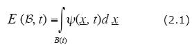
The integrand Ψ(ξ, t) which represents the extensive property per unit volume, is said to be the intensive property associated with the extensive property E. The main extensive properties considered in EOR models are the mass of different components, as well as the energy, contained in each phase of an EOR system.
A model of a macroscopic system is said to contain a shock when there is a surface, Σ(t), across which at least one of the intensive properties of the model is discontinuous. In our notation, Σ(t) will be the union of the surfaces across which the intensive properties are discontinuous. In particular, if the model does not contain a shock, Σ(t) is void. The kind of discontinuities that may occur across Σ(t) are 'jump discontinuities', exclusively. By definition, a jump discontinuity of a function is one in which the limits from each side of Σ(t) exist, but they are different from each other. Furthermore, the surface Σ(t) is oriented arbitrarily (i.e., a positive and a negative side are defined) and a unit normal vector, n, pointing towards the positive side is taken on it. The jump on Σ(t) of any function, f(ξ), is defined to be
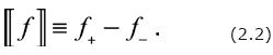
Here, f+ and f— are the limits on the positive and negative sides, respectively.
A Basic Axiom is: "An extensive property can change in time, exclusively, because it enters into the body. In turn, it can enter into the body through its boundary or directly in its interior." The mathematical expression of this Axiom is:
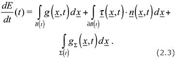
In these statements the amount that 'enters' may be positive or negative. With regards to Eq. (2.3), in the nomenclature of the general formulation of Continuum Mechanics, Allen et al. (1988), g (ξ, t) is called the external (distributed) supply of the extensive property and τ (ξ, t) is the flux of the extensive property. As for gΣ(ξ, t), it is also an external supply, but this one is concentrated on the surface Σ(t); see: (Herrera and Pinder, to appear). The function g (ξ, t) is the amount of the extensive property per unit volume per unit time that enters the body at the point ξ of the physical space at time t, while the function gΣ(ξ, t) is the amount of the extensive property per unit area per unit time that enters the body at the point ξof the surface Σ(t), at time t. The inclusion of such concentrated sources is essential in order to be able to treat shocks with sufficient generality; in particular, this will permit us to present in Section 5 an exhaustive description of shocks that may occur in Black–Oil models, which was originally reported in (Herrera et. al., 1993) and includes Buckley–Leverett's shocks (Buckley and Leverett, 1942) as well as those reported by Herrera and Camacho (1997) and Herrera et al. (1993). In particular, the double–discontinuity models of shocks occurring in variable–bubble–point systemsis an example in which, for some of the extensive properties that constitute the model, gΣ(ξ, t) ≠ 0 (Buckley and Leverett, 1942; Herrera et al., 1993; Herrera, 1996; Herrera and Camacho, 1997).
Finally, in Eq. (2.3), the function τ (ξ, t)•nat the point ξof the body external–boundary, ∂B(t), is the amount of extensive property that enters the body there at time t (Figure 1), per unit area per unit time. In EOR models, τ (ξ, t) represents the flux due to diffusion (mainly, material dispersion–diffusion or thermal diffusion).
A purely mathematical result (i.e., a mathematical theorem; see, Allen et al.,1988 and Herrera and Pinder, to appear) shows that Eq. (2.3) is fulfilled by each body of a continuous system, if and only if, the following 'balance conditions' are satisfied:

Eq. (2.4) will be referred to as the "balance differential equation", while Eq. (2.5) is the "jump condition". The systems of differential equations that constitute the mathematical models will be derived from Eq. (2.4), while the treatment of shocks will be based on Eq (2.5).
A unified model of EOR systems
Most EOR systems are multiphase systems, albeit there are a few that are one–phase systems. In any event, EOR systems are particular cases of the most general multiphase system treated in this Section. In the axiomatic approach that permits such a unified treatment any multiphase system is characterized by the following axioms:
1. A family of phases. Each phase of this family moves with its own velocity;
2. A family of extensive properties. Each extensive property of such a family is associated with one and only one phase; and
3. The basic mathematical model of the multiphase system is constituted by the system of partial differential equations and jump conditions that is obtained when the balance conditions for each one of the extensive properties of the family is expressed in terms of the corresponding intensive property.
Once the axioms of multiphase systems have been described in this very brief manner, what remains is to state them with greater precision in mathematical terms, as we do next. In particular, with respect to Axiom 2, the manner in which extensive properties are associated with phases requires being described in greater detail.
The number of phases and extensive properties of these families will be denoted by M and N, respectively. We observe that N≥M, necessarily. It is assumed that at each time, at each point of the physical space, there are M particles; each one of them corresponds to one and only one phase. Furthermore, given any domain of the physical space, let Bξ(t) be the set of particles of phase ξ (ξ may be 1,..., M) that are located at such a domain at time t. A family of M bodies {B1 (t),..., BM (t)} , is defined in this manner.
Then, a precise statement of the association between extensive properties and phases referred to in Axiom 2 follows. Given any extensive property Eα∈{E1,..., EN}, there is a unique ξ, to be denoted by ξ(α), such that it has the property

Clearly, here the range of α is {1,..., N}, while that of ξ is {1,..., M}. In Eq. (3.1), ψα is the unique intensive property associated with Eα. Thereby, we observe that corresponding to the family {E1,..., EN} of extensive properties, we have a unique family {ψ1 (ξ, t),.., ψN (ξ, t)} of intensive properties, since the correspondence Eα↔ψα, α = 1,..., N is one–to–one. Therefore, every intensive property is also associated with one and only one phase.
The global balance conditions for each extensive property Eα∈{E1,..., EN} can now be expressed, as follows (see Figure 2):
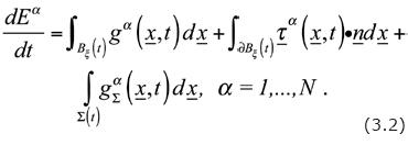
Here, it is understood(α) that ξ = ξ (α), where ξ corresponds to the unique phase associated with extensive property Eα. Furthermore, gα and gαΣ, are the 'supplies' of the extensive property a, the first one distributed in Bξ(t) and the second one concentrated on Σ(t), while τα is the 'flux' field of the same extensive property. The supply terms, gα and gαΣ, will also be referred to as the source terms. As was mentioned before, Σ(t) is the surface where discontinuities of any of the intensive properties of the model may occur;we observe that this definition is independent of the extensive property considered. However, for many extensive properties to be considered we will have gαΣ = 0, on Σ(t).
As it was seen in Section 2, the balance equation of any extensive property can also be expressed in terms of its corresponding intensive property by means of Eqs. (2.4) and (2.5). So, instead of the system of Eqs. (3.2), in what follows we use
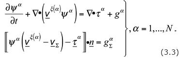
We recall that the jump conditions are fulfilled on Σ(t), while the differential equations everywhere, except at Σ(t) and the outer boundary of the continuous system.
This system of partial differential equations and jump conditions constitutes a unified mathematical model of EOR systems, which is the leitmotiv of the present article mentioned before; it includes exhaustively the mathematical models of EOR systems. In the remaining of this article, this general model is specialized to obtain the most commonly used models of EOR technology. In particular, we will obtain the models discussed in the very comprehensive and complete treaty of EOR models, authored by Chen et al. (2006).
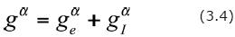
For models of EOR systems, it is useful to decompose the source terms gα (α = 1,..., N) into two parts whose origins can be traced back to the system exterior (gαe) and the system interior (gαI),respectively. Thus, we write
The black–oil model
The basic mathematical model of a Black–Oil system corresponds to the case when in the unified EOR model of Section 3, the following conditions are satisfied; the family of phases is constituted by:
1. A water–phase,
2. An oil–phase (liquid), and
3. A gas–phase.
In Black–Oil and isothermal Compositional Models the phase constituted by the solid matrix of the oil reservoir is usually ignored because it does not move and it does not exchange mass with the fluid phases.
There are three different substances (or components): water, nonvolatile oil (usually called 'oil') and volatile oil (usually called 'gas'), and only the volatile–oil may be in more than one phase; namely, the oil and gas phases. The family of extensive properties has four members:
1. The mass of water in the water–phase,
2. The mass of nonvolatile oil in the oil–phase,
3. The mass of volatile–oil contained in the oil–phase ('dissolved gas'), and
4. The mass of volatile–oil contained in the gas–phase.
Let ψi (i = 1,2,3,4) the intensive properties associated with each one of them. In this case the function ξ (α) is: ξ(1)=1, ξ(2)=2, ξ(3)=2 and ξ(4)=3. Then, the most basic mathematical model of Black–oil systems is given by Eq.(3.3); that is:

The jump conditions are:
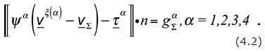
However, the jump conditionswill not be discussed in this Section; instead, in the next one they will be used for making an exhaustive analysis of shocks that may occur in Black–Oil models.
Explicit expressions, as integrals, of these extensive properties are:
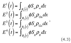
So, the corresponding intensive properties are

Furthermore, in what follows, we shall replace the superscripts 1,2,3,4, above, by w, Oo, Go and g, respectively.
Therefore, the basic system of differential equations of the Black–Oil model is constituted by the following system of equations
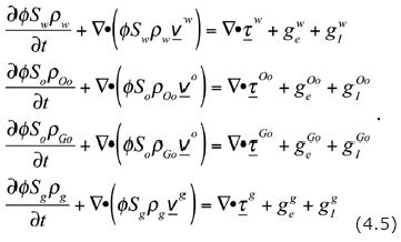
In the Black–Oil model dispersion–diffusion processes are neglected, so that τa = 0 (= w, Oo, Go, g). As for the internal sources, gαI, all them are zero except when α = Go, g. In the absence of chemical reactions, as it is assumed in the Black–Oil Model, the mass of volatile oil is conserved and then:

Hence, Eq. (4.5) reduces to:
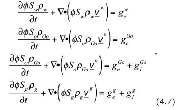
Generally, the external sources gαe are due to wells; they are negative if extraction occurs and positive if injection takes place. In particular, the terms —gwe and —gOoerepresent the mass of water and non–volatile oil extracted from the water and oil phases, respectively, while —gGoe and —gge represent the mass of nonvolatile–oil extracted from the oil and gas phases, respectively.
Starting with Eq. (4.7) it is easy to derive the standard forms of the mathematical model of Black–Oil reservoirs; in particular, for comparison we will use that presented in Chen et al. (2006). To this end we introduce the Darcy velocity, for each phase, which is defined by

Then, adding up the last two equalities of Eq. (4.7), we get

together with
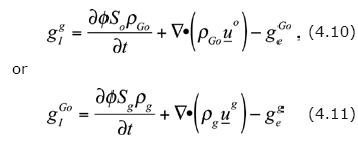
Eqs. (4.10) and (4.11) are not usually mentioned in the literature, since they are a sub–product of the methodology here applied for deriving the basic differential equations. However, they may be useful in some instances since either one of them can be applied for evaluating the nonvolatile–oil exchanged by the oil and gas phases.
The rest of the derivation is standard. Eqs. (4.9) can be transformed into (see Chen et al., 2006):
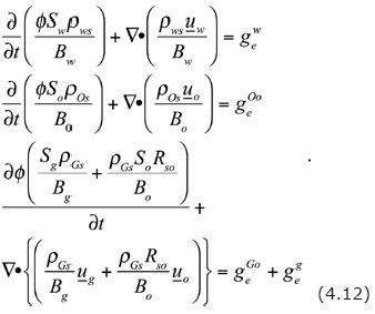
This is achieved introducing the following notation (further details of the symbols used here are given at the end of this Section):
The formation volume factors, Bw, B0 and Bg are defined by

Eqs. (4.12) have to be complemented by several constitutive equations relating the variables occurring in them. In particular, Darcy's law

the saturations identity
The capillary pressure equations
which relate the phase pressures. Both pcowand pcgo are functions of other parameters of the reservoir system, the saturations in particular, which must be determined in advance, experimentally or otherwise. The gas–oil ratio equation of state:

which is satisfied when Sg > 0; i.e., when the reservoir is truly a three–phase system.
The following list of symbols complements the notation already explained in the text of this Section:

From the mere fact that the system consists of three phases and one of them contains two components, while each one of the other two contains only one, without any additional knowledge, we have derived the system of equations given by Eqs. (4.1) and (4.2). Such equations give a very firm basis for incorporating all the scientific and technological knowledge available about the system, as we have done, to obtain as final product the mathematical model of Black–Oil systems.
Analysis of shocks that may occur in black–oil models
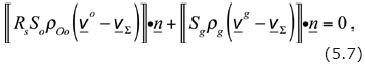
To start with, we observe that Darcy's Law implies that the pressure is continuous and, if the solid–matrix does not have abrupt changes in properties, as in the contact between two geological formations of different origin, the porosity is also continuous. Then, the shock conditions of Eq. (4.2) when the external source terms vanish can be written as:

where Rs(p, T)is the gas–oil ratio defined by ρGo = RsρOo.
A. In a region where the gas–phase is absent
The density ρOo is continuous across the shock Σ because so is the pressure po. When the gas–phase is not present Sg = 0, so that Eq. (5.1) implies  and implies

where the notation is such that for any function f,  is the the average of the function f across Σ.
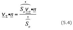
From the first equality in Eq. (5.1) it follows that when 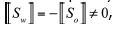 , the shock velocity is given by

On the other hand, from Eq. (5.2) it follows that when  , the shock velocity is given by
Generally,
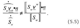
Therefore, if these two kinds of shocks coincide at any time they will separate, since their velocities are different. Thus, at a shock either  , in which case
 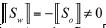 and the velocity of the shock is given by Eq. (5.3), or
  , in which case
  and the velocity of the shock is given by

B. At a gas front
For simplicity in what follows we only consider the case when the water phase is not present. At a front that advances into a region of under saturated oil, we take the unit normal vector pointing towards the under saturated region (Figure 3). Adding up the last two equalities in Eq. (5.1), one gets:
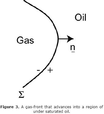
In the under–saturated oil region Sg = 0; i.e. (Sg)+ = 0, on Σ.
According to the second equality in Eq. (5.1), Σo(vo — v Σ) is continuous across the shock and therefore, from Eq. (5.7), it follows that

Using the identity 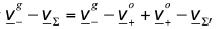 it can be seen that

With
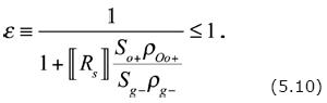
The physical interpretation of this result is that when a gas front advances into a region of under–saturated oil, it is retarded in its motion by the 'retardation factor' ε (see Herrera, 1996, and Herrera and Camacho, 1997).
C. In a saturated oil–region (Buckley–Leverett theory)
This is the case of a biphasic system in which the gas–phase and the liquid oil–phase coexist, which was treated by Buckley–Leverett in their classical theory (Buckley and Leverett,1942). In this case, because the oil is saturated and the pressure is continuous, Eq (5.1). reduce to

This is analogous to Eq. (5.2). Corresponding to Eq. (5.3), we now derive the equation:
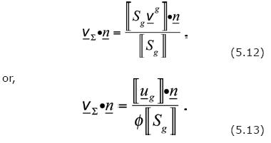
A special case of this equation is the immiscible and incompressible case considered by the classical Buckley–Theory, for which Eq. (5.13) becomes the well–known relation (see, for example, Herrera and Camacho, 1997):

Here,
The compositional model
In this Section we apply the general scheme of Section 3 to obtain the basic mathematical model of compositional oil reservoirs. The derivation need not be as formal as in Section 4, since the general protocol has already been illustrated there.
The characteristic features of compositional models are:
1. The family of phases is the same as before: the water–phase, the oil–phase and the gas–phase. The notation used for the velocities of such phases is also the same:
i) vw is the velocity of the water–phase;
ii) vo is the velocity of the oil–phase; and
iii) vg is the velocity of the gas–phase.
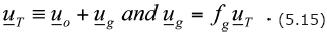
2. Besides the water, we distinguish Nc chemi–cal substances; these substances do not change chemical composition through time. However, through time, each one of them is exchanged by the oil and gas phases. The family of extensive properties consists of 2Nc + 1members; namely,
i) The mass of the water–phase, denoted by Mw;
ii) The mass of the i–th component in the oil–phase, denoted by Mio(t), i = 1,...,Nc; and
iii) The mass of the i–th component in the gas–phase, denoted by Mig, i = 1,...,Nc.
The notations used for the corresponding intensive properties, supplies (i.e., mass–sources) and flux–fields are:

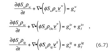
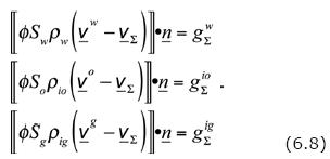
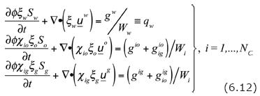
3. The basic mathematical model of the multiphase system is constituted by the system of partial differential equations and jump conditions of Eqs. (3.3); i.e.,
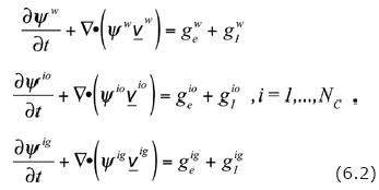
and

In Eq. (6.2), the source–terms have been expressed as in Eq. (3.4).
Eqs. (6.2) and (6.3) constitute the basic mathematical model of 'compositional' EOR systems.A model capable of predicting the system behavior, when it is subjected to suitable initial and boundary conditions, will be derived from it by incorporating sufficient scientific and technical information about the actual system following the protocol leitmotiv of this article.
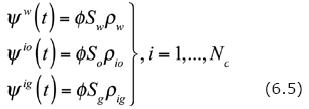
The integral expressions for each one of the 2Nc + 1 extensive properties are:

Therefore,
Furthermore, in the Compositional Model diffusion–dispersion processes of the components are neglected; this implies that all the flux–fields are zero; i.e.,

According to our assumptions  since no matter is exchanged with the water–phase.
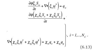
When all this is taken into account, the basic mathematical model for compositional systems, of Eqs. (6.2) and (6.3), becomes:
and
The contributions to gαe, α = w, io, ig, generally, are due to extraction or injection through wells. We observe that the following conditions are fulfilled:
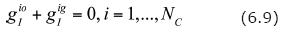
since the mass of each component must be conserved.
Mass interchange between phases is determined by the mass distribution of each component in the oil and gas phases through the condition of stable thermodynamic equilibrium (Chen et al, 2006). This condition is expressed by means of the equation
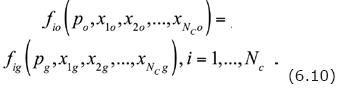
Here, fio and fig are the fugacity functions of the component in the oil and gas phases, respectively.
For the application of the stable thermodynamic equilibrium condition, the following notation and nomenclature is relevant:

Here, Ww and Wi are the "molar masses". On the other hand ξw, ξio, and ξig are the "molar densities" of the water, the i—th component in the oil–phase and of the i—th component in the gas–phase, respectively. Furthermore, ξα is the "molar density of phase α". The "mole fraction of component i in phase α", is χiα. Since the condition of stable thermodynamic equilibrium is expressed in terms of the mole fraction of component i in phase a, it is advantageous to express the basic equations of the compositional model in terms of such parameters. Then
Adding up the last two equalities appearing in Eq. (6.12) and using Eq. (6.9), we get
As in the case of the Black–Oil model, the last two equalities in Eq. (6.12), can be used to evaluate the supplies gioig and gigio due to exchange. We recall that for saturated flows, these equations are supplemented with the saturation identity:

Other equations that are applied in order to obtain a model capable of predicting the system behavior are:
Darcy's Law,

where krβ and μβ are the relative permeability and the dynamic viscosity of the b phase, and  is the absolute permeability.
Mole fractions identities,

Capillary relations,

here pcow and pcgo are the capillarity pressures of oil and water and gas and oil, respectively, and pβ is the pressure of the b phase. Equations (6.13)–(6.17), together with the stable thermodynamic equilibrium condition of Eq. (6.10) constitute a 2Nc+ 9system of equations for the 2Nc+ 9 dependent variables χio, χig, uα, pα and Sα, α = w, o, g, i = 1,...,Nc, which when subjected to suitable boundary and initial conditions provide a model capable of predicting the behavior of the compositional system.
The non–isothermal models
As stated before, in Black–Oil and Isothermal Compositional Models the phase constituted by the solid matrix of the oil reservoir is usually ignored because it does not move and it does not exchange mass with the fluid phases. However, the solid matrix cannot be ignored when formulating non–isothermal models since then energy balances have to be included and the solid phase plays a significant role in them. In turn, this is due to the fact that rocks and other materials that form the solid matrices of oil reservoirs have large heat capacities, frequently larger than the fluid phases participating in the reservoir systems.
Thus, the basic mathematical model of the non–isothermal compositional systems here discussed, has the general features that follow. The family of phases has four members: the solid matrix, the water–phase, the oil–phase and the gas–phase. The velocity of the solid phase is zero, while the notation used for the velocities of the other phases is the same that has been used in previous Sections. The family of extensive properties has 2Nc + 5 members. The first 2Nc + 1 are the same as for the Compositional Model. So, we only discuss here the other four; they are:
i) The total energy of the water–phase, denoted by Ew (t);
ii) The total energy of the oil–phase, denoted by, Eo (t);
iii) The total energy of the gas–phase, denoted by, Eg (t);and
iv) The total energy of the solid–phase, denoted by, ES (t)
For simplicity jump conditions will not be discussed. The differential equations required to complete the non–thermal compositional model are obtained applying Eq. (3.3). The total energy of each one of the phases is given by
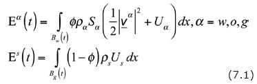
Where Uα is the specific internal energy (per unit mass) of phase a. Due to the smallness of the velocities occurring in flow of fluids through porous media, inertial effects are neglected and the kinetic energy is taken to be identically zero. Therefore, we take
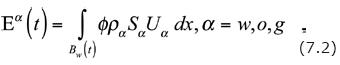
Using Eqs. (7.1) and (7.2) it is seen that the intensive properties that correspond to the total–energies of the different phases are

Since we are dealing with total energy, the energy sources should be decomposed into two parts: heat sources and mechanical–energy sources (Herrera and Pinder, to appear). A similar decomposition applies to the energy fluxes. This is better understood making the analysis in integral form. In such a form, the balance equations for the extensive properties associated with the different fluid phases (α = w,o,g) are:

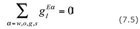
Here, the heat sources are: φαραhα and qαL . The former represents the rate per unit volume of the physical space at which internal energy is supplied to the a phase by sources distributed in the body–interior (due, for example, to exothermal chemical reactions), while qαL is the heat loss of the α phase to the overburden and underburden, also per unit volume of the physical space. The term —γρα(uα)z (γ is the gravity acceleration and (uα)z is the component of uα in the zdirection) represents the mechanical work done by the gravity force on phase α. Furthermore, we put together the exchange of energy between the phases in the term g EαI, which represents the total energy that enters phase a from other phases. As for energy fluxes that enter the α phase through its boundary, they are given by qα and  . The former is the heat flux, while the latter comes from mechanical work done on the boundary of a bodies. Finally, we observe that
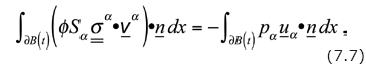
For the non–isothermal compositional model to be developed, the mechanical work done by the gravity force will be neglected (i.e., g(ua)z 0). Also, the work done by viscous forces will be neglected and, so, the stress tensor acting on phase a will be  . Therefore,

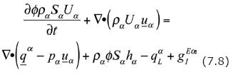
and Eq. (7.4) becomes
This balance equation, when expressed in terms of the intensive property, becomes
It can also be written as
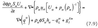
By definition, the "enthalpy per unit mass" of the fluid phase Hα (α = w, o, g), satisfies

Therefore, for α = w, o, g, Eq. (7.9) is

The balance equation for the extensive property associated with the energy of the solid phase is:

This balance equation, when expressed in terms of the intensive property, is:
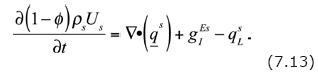
Adding up Eq. (7.13) and the four equalities of Eq. (7.11), we get

Here, we have applied Eq. (7.5) and written 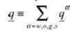 as well as
  . They are refe–rred to as total heat flux and overall heat source term, respectively.
A very important assumption that is made in the non–isothermal compositional model that we are presenting is that, at each point of the oil reservoir, the different phases reach thermal equilibrium instantly, which implies that all the phases have the same temperature, denoted by T, at each point. Then, the total heat flux is given by an overall Fourier Law:
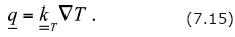
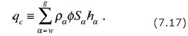
This leads to the following form, of Eq. (7.14):

Here, qc is referred to as the overall heat source term and it is defined by
Conclusions
Mathematical and computational models of the processes that occur in enhanced oil recovery (EOR) technology are fundamental for the application and advancement of such methods. At least the following three stages can be distinguished in the development of EOR models: construction of a mathematical, a numerical and a computational model, respectively. In particular, the construction of the mathematical model is the starting point and base on which the remaining construction is built. Due to the great diversity of processes occurring in EOR, it is valuable to possess a general and systematic procedure for constructing their mathematical models, which can be used as a unified protocol when building the corresponding computational simulators. In this paper we have presented such a procedure, based on an axiomatic formulation of Continuous Mechanics (Allen et al., 1988), which is systematic, rigorous and easy to apply independently of the complexity of the system considered.
As it is here explained, mathematical models of EOR processes are constituted by a system of partial differential equations together with a system of conditions, the jump conditions, which model discontinuities must fulfill when and where they occur; albeit, in standard treatments the jump conditions are not usually discussed. When building the mathematical model of an EOR system, the following stages can be distinguished: firstly, a basic system of partial differential equations and jump conditions that only depend on the number of phases and components in each phase are established —given in Eq. (3.3)–; and secondly, the phenomenology is incorporated into it. In this paper, the system of partial differential equations and jump conditions derived in the first step is referred to as the 'basic mathematical model'. This supplies a very sound and firm basis for a second step, which consists in incorporating other scientific and technological information that is required to complete the mathematical model; this latter purpose is achieved by means of certain number of constitutive equations such as Darcy's Law, chemical laws, results of field measurements and many more. Specific applications of the procedures here introduced have already been made in the development of EOR projects such as water–alternating–gas injection and air injection methods.
In standard approaches, the system of partial differential equations of the basic mathematical model is derived by means of balances that are carried out in cubes (or parallelepipeds) of the physical space, putting together the different phases of the system and the jump conditions are not usually discussed. In the protocol here proposed, on the other hand, such balances in cubes are not required since instead the starting point is the system of partial differential equations and shock conditions of Eq. (3.3). The procedure is systematic, rigorous and easy to apply independently of the complexity of the system considered. In Sections 4 to 6, we have shown that when this approach is used for constructing the basic mathematical models, such construction is to a large extent automatic; all what is required in order to define the partial differential equations and the jump conditions of the mathematical model is to identify the phases and species, as well the energy sources, that participate in the EOR system.
Bibliography
Akkutlu I.Y. and Yortsos Y.C., 2003, The Dynamics of in–situ Combustion Fronts in Porous Media, Combustion and Flame, 134, p.229–247. [ Links ]
Allen M.B., Herrera I. and Pinder G.F., 1988, Numerical modeling in science and engineering, John Wiley & Sons. 418 p. [ Links ]
Buckley S.E. and Leverett M.C., 1942, Mechanics of fluid displacement in sands, Trans., AIME, 146, p. 107–116. [ Links ]
Chen Z., Huan G. and Ma Y., 2006, Computational Methods for Multiphase Flows in Porous Media, SIAM. 549 p. [ Links ]
Chen Z., Ma Y. and Chen G., 2007, A sequential numerical chemical compositional simulator, Transport in Porous Media, 68, p. 389–411. [ Links ]
Herrera I. Shocks and Bifurcations in Black–Oil Models, 1996, SPE J. 1,1, p. 51–58. [ Links ]
Herrera I. and Camacho R.G., 1997. A Consistent Approach to Variable Bubble–Point Systems, Numerical Methods for Partial Differential Equations, 13,1, p. 1–18. [ Links ]
Herrera I., Camacho R. and Galindo A., 1993, Mechanisms of Shock Generation in Variable Bubble Point Systems, Computational Modelling of Free and Moving Boundary Problems, 2, Computational Mechanics Publicactions, Southampton & Boston, p. 435–453. [ Links ]
Herrera I. and Pinder G.F., Mathematical modeling in science and engineering, Wiley, 2011 (submitted). [ Links ]
Lake L.W., 1989, Enhanced Oil Recovery, Prentice–Hall, Englewood Cliffs, NJ. 550 p. [ Links ]
Noll W., 1974, The foundations of mechanics and thermodynamics (selected papers by W. Noll, with a preface by C. Truesdell), Berlin–Heidelberg–Berlin: Springer–Verlag, 324 p. [ Links ]

