


Servicios Personalizados
Revista

Articulo
 Inglés (pdf)
 Artículo en XML
 Referencias del artículo
 Enviar artículo por email
Indicadores
 Citado por SciELO
 Links relacionados
-
 Similares en
SciELO
Similares en
SciELO
Compartir

 Permalink
Geofísica internacional
versión On-line ISSN 2954-436Xversión impresa ISSN 0016-7169
Geofís. Intl vol.50 no.1 Ciudad de México ene./mar. 2011
Original paper
Simulating elastic wave propagation in boreholes: Fundamentals of seismic response and quantitative interpretation of well log data
Rafael Ávila–Carrera1*, James H. Spurlin2 and Celestino Valle–Molina1
1 Instituto Mexicano del Petróleo México, D.F. e–mail: cvallem@imp.mx *Corresponding author: rcarrer@imp.mx
2 Chokecherry Consulting Denver Co. USA e–mail: jimspurlin@comcast.net
Received: April 19, 2010
Accepted: November 11, 2010
Published on line: December 17, 2010
Resumen
Se presenta una formulación analítica orientada al entendimiento de la difracción, dispersión y atenuación de los modos de propagación en pozo. El principal objetivo de este artículo es el de comunicar y promover en la comunidad científica los fundamentos sobre la respuesta sísmica en la vecindad de pozos. Se considera una fuente puntual interna (monopolar y dipolar) y se presentan resultados novedosos de simulaciones comparando con datos reales. Una técnica importante que no ha sido ampliamente explotada en la investigación cuidadosa de la propagación de ondas elásticas en pozos petroleros es el registro de formas de onda sónicas. El tratamiento apropiado y el procesamiento adecuado de los sendos grupos de microsismogramas permiten la extracción de información útil en la caracterización y entendimiento de las formaciones de roca, y es crucial en la toma de decisiones dentro de la cadena de producción de hidrocarburos. En este trabajo se estudia la propagación de ondas en el pozo por medio de simulaciones numéricas con el "denominado" métododel Número–de–Onda Discreto aplicado a varios casos de pozos representativos en yacimientos mexicanos. Las contribuciones de esta investigación son: (1) evidenciar en los sismogramas el fuerte efecto de difracción y dispersión de ondas elásticas, aún trabajando en el caso homogéneo e isótropo, (2) describir en los dominios del tiempo y la frecuencia, la propagación de ondas generadas por una fuente puntual en un pozo cilíndrico lleno de fluido y (3) comparar resultados de simulaciones controladas con datos reales de registros geofísicos. Para validar nuestros cálculos se comparan historias de tiempo y curvas de dispersión contra formas de onda procesadas en profundidad para varios tipos de litologías. El grupo de resultados que aquí se reportan pueden ser útiles en el entendimiento y predicción de los efectos producidos por la presencia de fracturas y heterogeneidades sobre la propagación de ondas. Se espera que en un futuro cercano se establezca al modelado matemático de registros sónicos de onda completa como una técnica digna de confianza en la simulación e interpretación de datos de campo.
Palabras clave: propagación de ondas, pozos, difracción, modelado, registros sónicos de onda completa.
Abstract
An analytic formulation oriented to understand the diffraction, dispersion and attenuation of borehole propagation modes is presented. The main aim of this article is to report to the scientific community the fundamentals of the seismic response at the well neighborhood, excited by an internal point source and present novelty simulation results compared against real data. An important, but not widely exploited technique to carefully investigate the elastic wave propagation in petroleum wells is the logging of sonic waveforms. The appropriate treatment and adequate processing of such microseismograms allow the extraction of useful information to characterize and understand the rock formation and is crucial on taking of decisions in the hydrocarbon production chain. In this work, the study of borehole wave propagation is based in the performing numerical simulations with the so–called Discrete Wave–number method applied to various cases of representative wells in Mexican reservoirs. The contributions of this investigation are: (1) to evince in the seismograms the strong effect of diffraction and dispersion of elastic waves, even working with the homogeneous isotropic case, (2) to describe in frequency and time domains, the propagation of waves generated by a point source in a cylindrical borehole filled with fluid, and 3) to compare controlled simulation results versus real data from geophysical logs. To validate our computations, time histories and dispersion curves are compared with down–hole sonic waveforms for several types of lithologies. The set of results reported here may be helpful for understanding and predicting the effects produced by the presence of fractures and heterogeneities over the wave propagation. It is expected that in the near future, mathematical modeling of sonic waveform logs can be established as a trustworthy technique.
Key words: wave propagation, boreholes, diffraction, modeling, sonic waveform logs.
Introduction
Nowadays it is well known that geophysical well logs recorded at the shallow crust of the Earth exhibit strong random heterogeneities at observation ranges of short wavelengths. It is exact in such scale, where the study of multiple diffraction by cracks and heterogeneities becomes crucial, to correctly understand the phenomenon of wave propagation in complex rocks. The diffraction analysis by fractures, cavities, inclusions or vugs has numerous applications in engineering and geophysics. Some of these applications are: detection of cavities in civil engineering, locali–zation of fluid filled cracks and fractures in oil exploration and the description of cracks systems in hydrofracturing experiments (Baria et al., 1987, Stewart et al., 1981). Also, it is well accepted by the scientific community that the heterogeneous nature of fractured media is the main reason of several technical problems such as: excessive attenuation of waves in exploration seismology, in characterization of diffractors in seismic studies, variations on hydrocarbon production and its low recovery rates in petroleum industry, uncertainties in estimations of permeability and fluid saturation in flow problems, among others. Therefore, to understand the elastic behavior of a given fractured or porous media, it is necessary to determine the physical characteristics of such heterogeneities: geometry, orientation, spatial distribution, seismic response and spectral properties. Modern interpretation and exhaustive quantifications of such physical parameters can be made via wave propagation studies.
Seismic waves are affected mainly by porosity and the influence of elastic constants of the propagation media (Choquette and Pray, 1970). In addition, other parameters that affect the elastic wave properties are: fluid content, mineralogy and P–T conditions (Wang et al., 1991). The importance of mathematical models during the interpretation of data is illustrated in Stiteler and Chacartegui, (1997). They realized an analysis of synthetic seismograms that allows the quantification of wave edge effects and their multiples. Several studies in the field of modeling include attenuation and anisotropy explicitly (i.e., Carcione, 1995; Carcione, 1996(a), 1996(b); Carrion, et al., 1995). Other studies devoted to deal with porous media are: Carcione (1996(c) and (d)); Carcione and Quiroga–Goode, (1996(a) and (b)); Carcione and Seriani (1997) and Carcione and Tinivella, (2000). Several authors have studied the dispersion by inclusions using several numerical methods. Achenbach et al., (1978) worked on the research of the effects of a penny shape crack using shorter wavelengths than the crack dimension; examples with two cracks can be consulted in Bostrom and Eriksson (1993). Ávila–Carrera et al. (2006) and McMechan (1982) made the derivation for the characteristic resonances of a fluid filled cavity submitted to seismic excitation. Fehler and Aki (1978) and Fehler (1982) studied elastic wave interactions for a fluid viscous media, and the diffraction caused by a fluid filled fracture using a finite differences scheme (Chouet, 1986). The works by Bouchon (1985) and Campillo and Bouchon (1985) uses a method that combines a formulation of boundary elements and discrete wave number. In these works, the capacity to include arbitrary shapes of discontinuities has been demonstrated. Different techniques to establish statistical formalisms oriented to the generalization of results for properties in equivalent media have been used by Sabina and Willis (1989). The precision of numerical calculations of synthetic seismograms in bi– and tridimensional realistic models becomes a requirement for the characterization of fractured media. An arsenal of modern techniques is now available for this purpose (Ávila–Carrera, et al. 2009, Dorogoy and Banks–Sills, 2004, Frangi and Novati, 2003). This group of techniques corresponds to the so–called "Direct–Methods" where the Spectral Element Method (SEM) is distinguished by its usefulness and magnificent results. The realizations on the spectral approximation of wave equations in elastic and inelastic media for 2– and 3D complex geometries give this method multifarious applications and high precision calculations (Chaljub, et al. 2007). On the other hand, analytical and hybrid methods that combine the best properties of applied mathematics and numerical powering are needed (Godinho, et al. 2009).
The study presented here is based on the derivation, experimentation and test of a mathematical model. A discrete wave–number formulation was developed for this purpose. Wave propagation, seismic response and spectral characteristics produced by a monopole and dipole point sources were studied. Point sources were considered at the interior of a fluid–filled well embedded in an elastic, homogeneous and isotropic space. Fundamental aspects of wave physics, phase identification and velocities calculation are described for distinct reservoir examples in wells of the Faja–de–Oro, Mexico. The establishment of relations between petrophysical properties and results from the numerical simulations is essential. This tank is made by the analyses of raw data and synthetic modeling of sonic waveform logs. Results and explanations of dispersion and attenuation effects on synthetic sonic waves in slow, fast and very fast formations are reported.
Wave propagation at the well's neighborhood
Let us write an inhomogeneous wave equation with point source at the origin in 3D and harmonic dependence in time exp (iωt) as
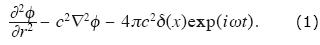
The solution to this equation for an elastic, homogeneous, isotropic and infinite space is obtained with the help of the potential f, which can be written as the displacement potential of an spherical wave affected by the decay of amplitude versus distance as
where  stands for distance to the observation point, and c = spherical wave propagation velocity in the fluid. The solution φ represents a spherical wave that propagates in the positive direction of R as depicted in Figure 1. To manage compact expressions of the Green´s function for displacements and stresses that contains mobile sources with constant velocity, eq. (2) is assumed to represent the scalar Green's function. It is possible to express this equation as plane wave decomposition by the way of the Weyl's integral (see Aki and Richards, 1980). Omitting the time term we obtain the following form
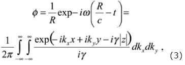
where kx and ky are respectively the components in x and y of the wave–number k = (kx, ky, γ), while the vertical wave–number is given by
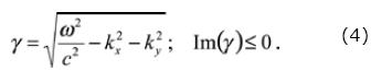
If we suppose that the source moves with constant velocity along the x–axis, we shall integrate over the entire domain of x–axis, taking into account the source position. This integration is performed as
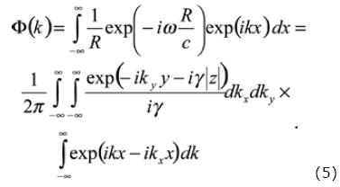
Solving the integration for a series of sources along the x–axis, we have that
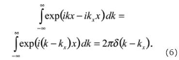
Equation (6) is a solution attributed to Lamb (1904). Thus, substituting equation (6) into equation (5) it is obtained
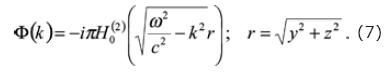
and substituting equation (4) into equation (7) we may write
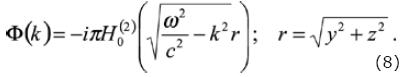
The integral from equation (8), represents the decomposition in plane waves of the irradiated wave field by the mobile point source. This equation can be expressed by Hankel functions using the Lamb representation and integrating over ky as follows
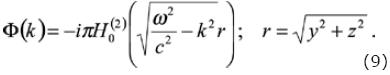
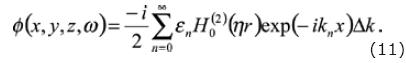
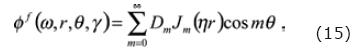
Expressing the eq. (9) as Fourier Series, we may write
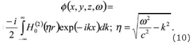
If we want to discretize the displacement potential of the source (incident field) then eq. (10) can be written as:
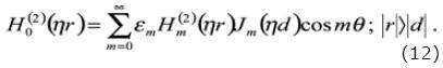
Then, can move the point source from the origin a distance d, as is depicted in figure 1, over one of the axes y or x, with the aim of having an eccentric source; we shall invoke Graf's addition theorem, and write
Finally, the displacement field generated inside the fluid–filled cylinder represented by p(r) is able to be expressed as the linear superposition of the point source and the diffracted (reflected) field by the borehole wall as
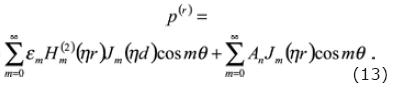
where: εm is the Neumann factor (ε0 = 1 and εm = 2 for m ≥ 1).
In the way, the expression for the displacements field (pressures) at the interior of the well has been obtained; it remains the formulation of the solutions for the entire space. Following this formulation is presented in a compact way.
In the frequency–axial wave–number domain, the diffracted field at the exterior elastic region (region S) is able to be expressed in a similar form as the incident field as
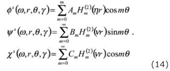
where the super index S, refers to the region where the potentials are evaluated and indicates that the value of the velocities at the solid must be used. The effective wave–number for the shear waves is v = (ω2/β2)—γ2; Im(v)<0. Am, Bm, and Cm are up to now, unknown coefficients that will be determined from the appropriate boundary conditions. Together with the factor expi(ωt—γz), the Hankel function of second kind and order m of the equation (14) can be read as divergent waves that irradiate energy forward to the elastic space. Because of the symmetry with respect to the x — y plane, equations in (14) involves both terms, sin(mθ) and cos(mθ), but not at the same time.
Despite the source position (internal or external in reference to the well), the diffracted (reflected) field in the fluid consist only of body waves. Such may be represented by
with the f super index indicating fluid.
The undefined constants Am, Bm, Cmand Dm from the eqs. (14) and (15) are obtained when continuity conditions of displacements and stresses at the fluid–solid interface are enforced, as uSr= ufr, σsrr= σfrr and σsrθ =σfrz = 0. Please note that as we assume a non–viscous fluid, the tangential displacements at the solid boundary (i.e., uSθ, uSz) have to be dissimilar from those in the fluid (i.e., ufθ, uzf). The enforcing of the four boundary conditions for each term in the m sum, allow us to conform a system of four equations four unknowns. This procedure is considered direct and it has been already treated by other authors. Therefore, we decide do not show it here. For the interested reader more detail about the classic Discrete Wavenumber (DWN) formulation can be found in Tadeu et al. (2001).
Once the coefficients have been determined by salving the system of equations, it is possible to compute the associated movements using the diffracted field in terms of standard equations relating the potentials and displacements. In essence, this requires the consideration of the equations (15) and (16) and also (13) for the case in which the source is considered at the interior of the fluid–filled borehole. Thus, we have to take into account the partial derivatives to convert potentials into displacements. Once this procedure has been performed, we are in the position to obtain expressions of the diffracted field at the solid and fluid regions in the following form
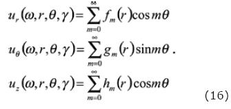
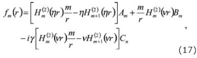
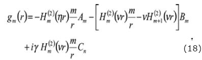
Where the functions fm, g m and hm are given by:
For the solid:
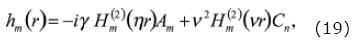
and for the fluid:
From these expressions we have to consider that just for the symmetry axis of the well and when m = 0, the terms are different from zero. Otherwise, at those points far from the axis of the borehole, the displacements are also function of the non–axisymmetrical terms with m > 0.
Fundamentals of Sonic Waveform Logs
In this section full waveform sonic logs are conveniently reviewed. Our attention will be focused on the Dipole Sonic Waveform Logs. Among other tools and trademarks, nowadays the Dipole Shear Sonic Imager DSI represents one of the main tools employed in petroleum industry and exploration geophysics to directly determine elastic and propagation properties. This is accomplished by making measurements of the pressure field varying in function of the time at the interior of an exploration well. Among the several possible applications of the mathematical formulations previously presented, there is the correct interpretation and quantitative simulation of some field logs. These logs are recorded with sonic tools from geophysical well logs. Thos wise, we consider appropriate to make a short review of the Monopole and Dipole Sonic Logs before the presentation of synthetic simulations of the field data.
The DSI tool combines the new dipole technology with the latest developments of the monopole measurement in a single system (Haldorsen et al., 2006). This tool offers one of the best methodologies available nowadays to obtain slownesses of P–, S– and Stoneley–waves. The slowness is equal to the inverse of velocity, and corresponds to the transit time given by the conventional sonic tools.
The Dipole technology allows the measurement of shear–waves in "soft" and "hard" rock formations, having some limitations due to the physics of the well. The monopole tools are able to detect shear–wave velocities greater than the velocity of the fluid in the well ("Fast–formations"), in other words, just S–waves velocities in "hard" rocks. The DSI now surpasses this fluid velocity limitation.
The DSI is a multi–receptor tool with a linear array of eight receivers, one monopole and two dipole transmitters. The receivers array enable to obtain more spatial samples of the wave propagation field to perform a full waveform analyses. The array design between transmitters and receivers allows the measurement of wave components that propagate beneath the formation.
One of the new characteristics of the dipolar sonde is the acquisition of Stoneley–wave velocities. A monopole energy source of low frequency to acquire high quality measurements of Stoneley–waves is utilized. The permeability derived from the Stoneley–wave is useful for evaluating cracks and to enhance the deep of investigation in the formation. DSI also represents a new technique to detect the compressional–wave arrivals and this measurement is compatible with previous sonic logs. The vertical resolution of the P–wave of the sonic log is six inches (0.1524 m). To determine slowness values for P–, S– and Stoneley–waves, an array of fast velocity processors that uses the Slowness–Time–Coherence method (STC) is employed (Kimbal and Marzetta, 1984). A band–pass group of filters optimize the frequency range for each propagation mode. The process provides no–ambiguity transit times even at the most difficult conditions in the well. The results are then useful input data for the determination of mechanical properties, formation evaluation and seismic applications. In addition, the DSI tool is totally compatible with previous sonic logs, offering substantial reduction in times and sonic conventional measurements at open or cased holes.
The mechanical properties of the rock can be characterized by the bulk–density and the elastic dynamic constants. These constants control the propagation velocity of P– and S–waves (Body–waves). In fluid saturated rocks, these properties depend on saturation percentage, fluid type, array between the grains of the rock and intergranular cementation grade. "Soft" rocks or poorly consolidated, exhibit low stiffness values. In a "slow–formation" the shear–wave velocity of the formation is lower than the fluid velocity, this is, Vs < Vf . As a result, the sonic waves travel more slowly in "soft" rocks.
Monopole logging tool
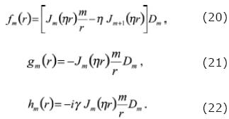
In the conventional sonic tool (Monopole), an omni–directional source creates an impulse of compression in the borehole fluid which propagates towards the formation. At the time that the pulse enters into the formation, a light but uniform bubble of compression is created around the well as shown in Figure 2. In consequence, compression– and shear–waves are excited and body–waves travel into the formation; head–waves are generated in the fluid of the well. These are the body–waves modes that are detected by the receivers instead of P– and S–waves of the formation. The phenomenon is illustrated in Figure 3. A logging diagram of eight traces for an example corresponding to a "hard"/compact formation in a well at the Faja–de–Oro, México is shown. The arrival of different propagation "phases" is notorious. The phase velocities can be directly read from the micro–seismogram. P–, pseudo–Rayleigh– and Stoneley–waves are clearly appreciated in the seismogram. Corresponding amplitude spectra have been calculated (Figure 3, top) in order to support the mode characterization. Smoothed Fast Fourier Transform (FFT) of each trace is represented by solid lines in the spectra. Three spectral peaks can be identified. Those peaks are the three characteristic frequencies and imply three propagation modes. In particular, 6 kHz (Stoneley–), 10 kHz (pseudo–Rayleigh–) and 13 kHz (P–waves) are encountered. Generally, those maximum amplitudes represent the resonant frequencies of each mode. The maximum spectral ordinates are the conspicuous resonant peaks in which the propagation of each mode is optimum.
The "so–called" head–waves are created when the body–waves propagate upwards through the well and travel faster than the waves propagating in the fluid. The P–waves in the formation are always faster than the waves in the fluid. In contrast, it is not ever the case for S–waves (or Pseudo–Rayleigh). In slow–formations or poorly consolidated, the shear–wave velocity is usually slower than the fluid velocity. Even though, both the body compression–wave and its head wave in the fluid exist; the S–wave perturbation will occur at the borehole wall and no head wave will be generated. In such particular case, the compression and fluid modes constitute the inherent information carried by the waveform.
Moreover, the guided waves (head– and Stoneley–waves) are the most complicated ones, since they are originated from trapped reflections of the source in the well and both types of waves are highly frequency dependent. Also, the Stoneley–wave is a superficial guided mode that propagates more slowly than the waves in the fluid.
Dipole logging tool
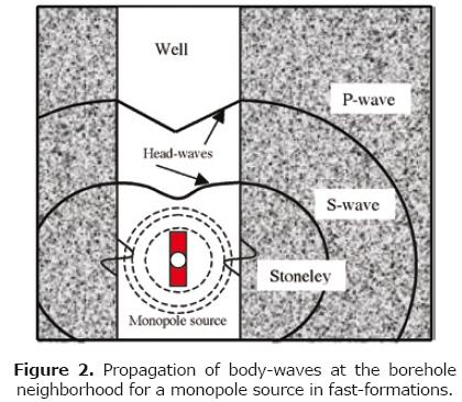
The Dipole tool uses two perpendicular directional sources and two sets of (in–line and cross–line) receiver arrays. The description provided here avoids the cross dipole operation mode. The dipole source behaves like a piston, creating a pressure increment over one side of the well and a decrement of pressure on the other side. This effect causes a small flexion at the borehole wall, as is illustrated in Figure 4. Also, the source excitation directly creates compression– and shear–waves into the formation.
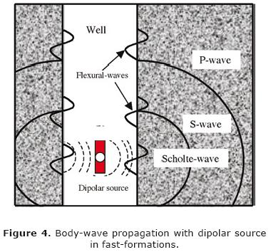
In addition, the flexural–wave propagation is coaxial in the well, while the displacements occur at angles of 90° with respect to the symmetry axis of the borehole (inline with the transducer orientation). The source works in the range of low frequencies, usually below 4 kHz, where the excitation of these modes is optimum. However, there is a new source option which operates under 1 kHz. With an improvement in the signal to noise ratio, above the 20–dB, this kind of source offers good results at large holes and very slow–formations. Thus, the depth of investigation can be increased.
Although, P– and S–waves irradiate energy directly into the formation, there are shear/flexural–waves added to the upward propagation in the well (see Figure 4). This effect creates a pressure change of a "dipolar type" in the fluid and the difference of pressure is what directional receivers detect. The shear/flexural–wave, caused by the bending action of the borehole, is dispersive and travels at low frequencies with the same velocity of the shear–wave; in contrast, the propagation velocity diminishes at higher frequencies. Contrasting with to the monopole conventional tools, the dipole tool allows measurements of the shear/flexural–wave even at slow–formations.
In slow–formations the shear/flexural–wave has short duration and concentrates in the range of low frequencies. Besides this wave, a compression–wave arrival of high frequency occurs and it is recorded at the beginning of the micro–seismogram. These packages of waves are called "leaky P–waves" (Pistre et al., 2005) and will be extensively described in the following sections.
Figure 5 (bottom) shows a waveform log for dipole source in fast–formations recorded at a well in the Faja–de–Oro production zone. The eight traces of low frequency content (2.2 kHz) clearly show two packages of waves. This observation is corroborated by the Fourier amplitude spectra for each trace plotted at the top of Figure 5. Also, two characteristic frequencies at 1.3 kHz and 3.2 kHz are observed. The maximum spectral ordinates represent the two conspicuous resonant peaks for two propagation modes, respectively. Identification of flexural– and tube–waves may be possible at this stage. However, discrimination of tube–waves is out of reach with this process by itself. On the other hand, in Figure 5 (bottom) the waveforms are characterized by a first set of arri–vals at 2.0 ms to the shorter offset receiver. Here is the flexural dispersive mode that propagates near to the shear–wave velocity of the formation (Vflex= Vs ± Vs *.14). We encourage the readers to directly measure this velocity from the micro–seismogram of Figure 5. A second group of waves is remarkable in the micro–seismogram after the flexural–wave arrival times. This dispersive mode corresponds to the tube–wave that is produced by the shear mode at low frequency and propagates as Sholte– or Stoneley–wave. Other possible interpretation of the arriving phases after the first move–out of flexural waves is given by the analysis of dispersion curves, where it can be appreciated that both, the first superior mode of flexural waves are propagating at same frequencies with Stoneley– or Scholte–waves. The unique tracking difference is the propagation velocity. Detailed review of dispersive waves will be addressed in the following sections.
Modeling results and quantitative interpretations
A central objective of this investigation is the comparison of numerical simulations with real well data. In other words, the principal aim is to synthetically rightly reproduce and mimic some groups of waveforms logged in homogeneous and isotropic formations. The calibrated numerical model can be used to study the variation of the seismic responses for heterogeneous and more complex formations under several well conditions. To asses the results from synthetic micro–seismograms using the mathematical formulation developed in this work, some sonic waveform logs observed at Mexican exploration wells are used. A single set of wells with different elastic properties in the mud/formation contact were selected to perform the modeling. Particular observations were reproduced varying the physical characteristics of the rocks, such as: size, bulk–modulus, hole–quality and compactness. For completeness of the set of results a first set of 2D examples were successfully obtained.
Figure 6a shows synthetic traces of the radial displacement field over time and the complexity of the seismic response at the well neighborhood is clearly observed. Fifty one receivers virtually disposed in the elastic space at coordinates y=2a and —3a ≤ x ≤ 3a are depicted. The monopole point source is located at the origin, as indicated at left hand side of same figure. The normalized properties of the fluid are a fluid compression velocity of αf = 1.0 and a fluid density of ρf = 1.0; and in the elastic solid we have αE= 2.0, βE= 1.0 (compression and shear wave velocities, respectively, and a density of ρE= 1.0. In this experiment it is clear to observe how the source located at the center of the model produces predominately P–wave propagation inside the fluid and through the elastic media. The model is axi–symmetric and only P–wave propagation modes can be generated.
Figure 6b presents the synthetic seismograms for the model at left with an eccentric point source x = 0.5a. The receiver distribution and the elastic and acoustic properties in the well and the surrounding media are similar to those reported in Figure 6a. The big differences between results of Figure 6a and Figure 6b can be clearly observed. In the last one, the presence of converted wave modes (S–waves) that travel at low velocities in the elastic media is evident. Such behavior is caused by the interaction between the eccentric source point and the borehole wall. These modes are also called "creeping–waves" and are denoted as P1, P2, P3 for consecutive arrivals of P–waves and C1, C2 and C3 for the creeping– (converted–) waves arrivals, respectively. Now the movement inside the well is asymmetric; generating new wavefronts that are immediately behind the first arrival of the original field of P–waves. Beside a clear trapping effect of energy in the well, there is an image response at 2.6 ms observed by the receivers located at the negative flank of the x–axis. This is due to fluid resonance given by the high contrast of elastic and acoustic properties in the model.
Tree dimensional synthetic computations for slow–, fast– and very–fast–formations are reported in this section. The synthetic micro–seismograms were calculated using a computer code that solves the wave equation in polar coordinates. Diffracted wave field in a cylindrical homogeneous well with a centered point source in 3D are calculated (Tadeu et al., 2001). This is the codification of the DWN formulation described in section 3. The model is constructed as a problem of diffraction of elastic waves produced by a monopole point source in the fluid. The source is located at the center of the well. The receivers are disposed above the source, aligned along the vertical axis with the same spacing among them (see Figure 1).
At the interior of the well, the propagation media is defined as elastic, homogeneous and isotropic. The purpose is to study the pressure field produced in the fluid due to the presence of the borehole. Also, multi–component total displacements fields are calculated at any place in the model by means of the Graff addition theorem. The synthetic micro–seismograms are calculated by spectral convolution and the intervening terms are the Transfer Function obtained by the model and the excitation function given by the Ricker wavelet or a Blackman Harris pulse (Kurkjian, 1985). In this way, with the help of the Fast Fourier algorithm, it is possible to synthesize the responses in time domain. In what follows, examples for data and models that use monopole and dipole sources are presented.
To render synthetics results useful to interpret real data, it is convenient to select an interval in the DSI log where a good quality waveforms are encountered. In other words, a well section that presents high quality phases of P–, S– (Pseudo–Rayleigh) and Stoneley–waves. It is desirable that the rock formation is competent, this is, good hole and good STC processing results. STC process is fundamental in the selection of the group of waveforms and the studied interval. When contour groups are well defined in the STC diagrams and other information from the suite of logs is available in the selected interval, performing the modeling is very attractive. It is important to keep in mind that despite that our model can reproduce many of the observed parameters in the real data, some conditions in the well as: pressure, temperature, heterogeneities and anisotropy of the formation are not considered. Furthermore, the knowledge of the limits and restrictions of the model augment the probability of success. The matching between the model response and the observed waveforms directly depends on the optimum selection of input parameters.
The computations involved six input parameters, which are obtained principally from the previous STC processing on the acquisition waveforms to be modeled. These input quantities are: P–wave velocity of the formation Vp, S–wave velocity of the formation Vs, density of the formation r, velocity in the fluid Vf, density of the fluid rf and radius of the well ρf. The propagation parameters are obtained directly from the STC diagrams, while the hole radius is a conventional parameter, the fluid density is obtained from perforation logs and the density of the formation is extracted from the porosity log.
The micro–seismograms in Figure 7 correspond to a synthetic waveform (top) and to a single receiver full waveform observation (bottom). Data were obtained from a typical fast–formation well from the Faja–de–Oro reservoir. To be modeled, the first receiver of the array was chosen to obtain the best signal/noise ratio. The parameter values used in the model are: Vp = 2930 m/s, Vx = 1,437 m/s, Vf = 1,088 m/s, ρ = 2.37 g/cm3,ρf= 1.4 g/cm3 and r = 0.177 m. A good agreement between the two traces can be observed. Firstly, the P–wave arrival that appears immediately behind the origin time in the observed trace is not shown in a defined way by the synthetic trace. However, the S–wave (Pseudo–Rayleigh–wave) that appears in the observed log later than 1.0 ms, is accurately reproduced by the synthetic trace. The arrival time of the synthetic Pseudo–Rayleigh–wave is close to the original S–wave. The next phase, even with less amplitude, is clearly identified in the synthetic result with some delay with respect to the original arrival time. Secondly, the relative amplitude between Pseudo–Rayleigh– and Stoneley–waves from the original signal is well reproduced by the synthetic trace. Looking forward, the corresponding phase change from Pseudo–Rayleigh to Stoneley has been pointed out with a black arrow in Figure 7. This feature remarks the good reproduction by the synthetic log. Finally, another fact of good simulation is the capability of the synthetic log to efficiently mimic the amplitude coda decay for both phases, Pseudo–Rayleigh and Stoneley. The matching of codas for the Pseudo–Rayleigh–waves is very good. Numerical reproduction of the coda decay for Pseudo–Rayleigh and Stoneley phases is crucial to understand the attenuation values. Otherwise, data observation indicates that geometrical spreading is dominant in this example. Non viscous damping operator has been included in the DWN formulation.
Figure 8 shows the synthetic waveform (top) and observed (bottom) obtained for a very fast formation. The values of the elastic properties are comparable with that equivalent to a rigid borehole given the high velocity contrast between the solid and the fluid. The parameter values used in the model are: Vp = 6,220 m/s, Vx = 3,242 m/s, Vf = 1,604 m/s, ρ = 2.55 g/cm3,ρf= 1.0 g/cm3 and r= 0.1016 m. It is possible to observe the great similarity of the two traces. Despite the lack of definition of the P–wave arrival in both micro–seismograms, the agreement in the first group of P–waves that appear before 1.0 ms is noticed. This first set of waves is reproduced in the synthetic trace satisfactorily. Nevertheless, there is a small discrepancy for the arrival time of both micro–seismograms. The Pseudo–Rayleigh–wave that arrives at 1.8 ms in the data is promptly preceded by the Stoneley–wave. This tube wave is interacting with the S–wave and its arrival time is not clearly appreciated. However in the synthetic trace, the Stoneley–wave is very clear and eminently precedes the phase of Pseudo–Rayleigh. This result shows certainly that the Stoneley phase is almost immersed into the Pseudo–Rayleigh–wave. Such effect can be observed in the real waveform. It is important to notice that the relative amplitudes among P–, Pseudo–Rayleigh– and Stoneley–waves, observed in the original trace are reproduced with good accuracy by the synthetic trace. Finally, despite the poor reproduction of the Stoneley–wave Coda by the synthetic trace, the amplitude decay for the Pseudo–Rayleigh–wave is very similar with respect the original trace. It is remarkable to note the presence of late arrivals of Coda–waves in the observed signal that are attributed to trapped energy from the scattering of shear–waves (Aki and Chouet, 1975). This coda energy is not reproduced by the synthetic result. The amplitude decay of the Stoneley–wave coda in the observed log is of great importance due to its direct relation with the presence of cracks and heterogeneities in the formation.
The presence of several technical features in the synthetic micro–seismograms is encouraging to obtain a good representation of real waveforms. In the following, it is proposed a list of fundamental characteristics with the aim at obtaining a good reproduction and better understanding of real data. Without rigorous detail, a good synthetic log should have acceptable approximations on: 1) arrival times of different phases, 2) propagation velocity, 3) relative amplitudes among the phases, 4) frequency content and 5) energy decay and duration.
Figure 9 shows the comparison between the synthetic micro–seismogram computed with the DWN model of the fluid filled well with a point source at the origin (Figure 1) and the full waveform responses from the DSI log in a fast–formation. The data were selected from the suite of logs in a well at the Faja–de–Oro Mexico. The input parameters used for computations are: Vp = 2,930 m/s, Vx = 1,437 m/s, Vf = 1,088 m/s, ρ= 2.37 g/cm3,ρf= 1.4 g/cm3 and r= 0.177 m. As reference, we can see from the available petrophysical report that the formation interval of interest is described as good consolidated homogeneous sandstone. The good quality of logs and the constant value of the caliper indicate this well section is a suitable candidate to be modeled. In both micro–seismograms of Figure 9, the amplitude displacements of eight vertical aligned receivers separated by Δz = .1524 m are plotted versus time. The source–first receiver distance (offset) is 2.74 m = 9 ft.
In general, there is good agreement in the waveforms of both graphs. Regardless the lack of definition of P–wave arrival times in both graphs, the Pseudo–Rayleigh–wave arrival is reproduced accurately by the synthetic traces. This train of waves is well reproduced along the profile of micro–seismograms. The arrival time around 1.0 ms and the move–out that presents the shear–wave propagation velocity are rightly emulated by the traces computed numerically. Alternatively, the relative amplitudes and frequency content observed in the DSI data have also been well approximated. The synthetic reproduction of Stoneley–wave appears to be delayed by 0.5 ms with respect to the observed arrival time. However, the amplitudes of Stoneley–wave seem to be reduced in some traces. The amplitude decay of the synthetic tube–wave through the space (geometrical spreading) has a better representation in comparison to the temporal decay of the Coda. In turn, the synthetic coda for Pseudo–Rayleigh phase exhibits an excellent match with observations.
The selected temporal excitation function in the model corresponds to a Ricker's pulse. The phase and period values of this pulse have been arbitrarily controlled to obtain more accurate results. A priori, it is known that this time wavelet is different from the time function used by the tool. Unfortunately, the monopole transmitter time function is not published by the service company. Ricker's or Blackman Harris's wavelets are sufficient to closely approximate the synthetic reproduction of the observed traces.
Figure 10 depicts a new comparison between synthetic results and observed full waveform sonic logs for a very–fast formation (Vs>>Vf). At the left–hand side the numerical simulation of wave propagation for the model of Figure 1 is elucidated. The following values were employed for the computations: Vp = 6,220 m/s, Vx = 3,242 m/s, Vf = 1,604 m/s, ρ= 2.55 g/cm3, ρf = 1.0 g/cm3 and r= .1016 m. Again, eight vertically aligned receivers with separation of Δz = .1524 m are plotted. The offset is 2.74 m = 9 ft. The extraction of these parameters is coming from the previous STC data processing. According to other log information, the selected formation interval corresponds to a well section in a hard rock with presence of fractures saturated with fluids. Although the complexity of the evaluated formation, the results of synthetic traces are encouraging. The correspondence of respective arrival times and slopes of the move–out for the different phases is notorious. For instance, despite the fact that P–wave arrival is not observed in the data; a clear and good defined P–wave train around 1.0 ms is reproduced by the synthetic traces. Hence, it is possible to search for the P–wave arrivals in the data. It is also noted that a good representation of the Pseudo–Rayleigh–wave is achieved. The relative amplitudes, frequency content, propagation velocity and move–out are almost identical those presented by with the data. It has to be pointed out from observations, that the Stoneley–wave is found immediately behind the Pseudo–Rayleigh phase. The same effect is presented in the resulting traces from modeling, which reinforces the fact that the physics of propagation in the well is the cause of such phase interaction. A clear identification of the Stoneley–wave can be seen around 1.6 ms in the synthetic micro–seismogram. A strong arrival of this phase is identified after the Pseudo–Rayleigh–wave. The definition of the arrival time and propagation velocity for the Stoneley–wave in the data is not an easy task. It is difficult to locate the beginning of the Stoneley mode or the ending of Pseudo–Rayleigh. However, to elucidate this controversy, the arrival time and the move–out in the simulated Stoneley–wave are defined.
Furthermore, the relative amplitudes for each analytic trace of the inhomogeneous phases —Pseudo–Rayleigh and Stoneley— are comparable with those observed in the waveforms. The decay by geometrical spreading is another element that successfully has been reproduced. The spatial response of the receivers represents satisfactorily the dispersive wave field versus distance.
From the results of Figure 10., the simulations of the Coda decay for the inhomogeneous phases have to be refined out in the near future. The studied rock formation contain fractures, fluids and very high velocities, and it is well known that the main content of the coda energy occurs as an effect of the heterogeneous media (Lee et al., 2009). Despite the fact that our computations have no advantage to take into account the inclusion of irregularities, scatterers or fluid elements; the simulated traces appear to be accurate. The mismatch obtained by the slow–formation numerical experiments does not allow us the publication of high quality results. The main reason of the mismatch is that the basic formulation works properly only for a fluid filled well embedded in an homogeneous elastic solid.
Dispersion characteristics
The propagation and dispersion characteristics of guided waves in a fluid filled well with a centered point source are reviewed in this section. Synthe–tic computations of sonic waveform logs and dispersion curves are employed to this purpose. The dispersion characteristics for P–, Pseudo–Rayleigh– and Stoneley–waves with a monopole source are obtained using the analytical formulation presented in this paper. Similar results are obtained for Flexural– and Pseudo–surface–waves in a well model containing a dipolar source. The borehole effective radius becomes an important factor that governs the relative amplitudes of the synthetically generated modes. The Poisson's ratio in the formation is the primary factor on the determination of relative amplitudes of porous modes (leaky), present as consequence of propagation of compression waves in slow–formations. Attenuation affects both, duration and decay of the guided–wave modes. Once the model has been established, dispersion curves are calculated by the way of amplitude inversion and search of the minimization of errors. To cope with the huge variety of numerical methods to predict the linear phenomena behavior, a modified Prony's method is used here in order to extract relevant information from the wave–fronts of different propagating phases. Prony's method is a non–linear numerical technique to model digital data in terms of the combination of exponentials (Marple, 1987). However, it is not a spectral approximation technique and has a closer relation with those linear prediction algorithms used by recursive estimation operators. In addition, Prony's method searches the matching of an exponential deterministic model to the data. The philosophy behind is to utilize a least–squares analysis to approximately adjust an exponential model for cases where the number of data exceeds the inferred exponential terms.
Now we present dispersion processing results for synthetic logs generated by the homogeneous model in a fluid filled well for slow–, fast– a very–fast–formations. For monopole and dipole logs, the following parameters were employed in the computations of corresponding dispersion curves. In the model with monopole source: N=512 stands for number of samples by trace, Δz=10x10–6s stands for time sampling rate, Nf=200 stands for number of frequencies, Nr=24, 32, 64 stands for number of receivers for slow–, fast–, and very–fast–formations, respectively. Δz=.1524/3, .1524/4, .1524/8 m stands for spatial sampling rate for slow–, fast–, and very–fast– formations, respectively. For the model with dipole source: N=512, Δt=40x10–6s, Nf =200, Nr=24, 32, 64 and, Δz=.1524/3, .1524/4, .1524/8 m, respectively. An additional advantage of numerical simulations is that the parameters involved can be modified with great flexibility. For instance modification of the number of receivers, the spatial sampling rate and the number of samples can be handled by the inversion method toward the enrichment of the output.
Figure 11 depicts the dispersion curves resulting from the processing of six sets of synthetic waveforms. The diagrams of frequency versus slowness for monopole source (left) and dipole source (right) in slow–, fast– and very–fast–formations are presented. The constant solid lines in red, green and blue, are the P–wave slowness Δzc, shear–wave slowness Δzs and mud slowness Δzm, respectively. These constant lines are computed by setting to zero the matrix determinant in the inversion method. In other words, the source term is not included. The cut–wrapped curves correspond to the Aliasing effect. This shifting curve effect is due to the Nyquist frequency consequence of short number of samples. The short red dashed lines are the exact dispersion curves computed theoretically. The parameters used to obtain the synthetic traces and their corresponding dispersion curves to the slow–formation are: Vp = 2,257 m/s, Vs = 952 m/s, Vf = 1,604 m/s, ρ= 2.05 g/cm3, ρf = 1.0 g/cm3 and r= .203 m. As is illustrated in Figure 11 (top–left), the velocity Vs<Vf difference and the high contrasts in slow–formations cause the propagation of leaky–P–waves also called "porous modes" in the case of monopole source excitation. The mode that propagates at low frequencies is the compression normal mode. The slowness of this mode ranges from that of the P–slowness of the uninvaded formation and the cut frequency, to the mud–slowness at high frequencies. The following modes are compression superior modes of propagation. It is also characteristic the observation of dispersion curves patterns well marked and continuous. Up to five tendencies of events (black dots) shows that highly dispersive superior propagation modes can be followed. The leaky modes are featured by their complex wavenumber or complex frequency and their diffusive loss of energy in packages. Literature has reported this phenomenon as the result of combining interaction of trapped waves with the borehole wall and the high contrast in the Poisson's ratio. On the other side, the inversion process is able to detect porous–waves given its good precision. Despite the poor resolution in the data processing for eight traces, the inversion results can be improved growing the number of receivers in the synthetic micro–seismograms.
Similarly, the dipole results (Figure 11 top–right) display P–wave propagation porous modes varying from compression–slowness at low frequencies up to mud–slowness near 12 kHz. As seen, these modes exhibit a wide range of frequency content.
In addition, an extra mode is concentrated at low frequencies and high slownesses (slow velocities) for the dipole source. This mode corresponds to the Scholte–wave and exhibit dispersive behavior, which is generated by the low–frequency shear mode propagating as a tube wave. Also, the Scholte–wave propagation can be interpreted as the continuance of the flexural fundamental mode, since there is a gradual velocity reduction towards the high frequencies. In this way the Scholte–wave is defined, specifically when the low limit of mud velocity is exceeded. This concept is valid due to high dispersion content of the flexural mode. The corresponding time response will be a flexural fundamental mode, followed by a linear combination of Scholte and flexural first superior modes as depicted in Figure 5. Some P–wave components at high frequencies greater than 10 kHz can be found also.
The model parameters to the fast–formation (Figure 11– middle) are the same of those of Figures 7 and 9: Vp = 2,930 m/s, Vx = 1,437 m/s, Vf = 1,808 m/s, ρ= 2.37 g/cm3, ρf = 1.4 g/cm3 and r= .177 m. Such values were tied with the well suite log report. We have to remark that a well logged with an oil based mud (OBM) is sufficient result in changing the Vs/Vf contrast. Thus, a slow–formation in a water–based–mud well might behave as a fast–formation in OBM. The fast–formation example here represents the case of a homogenous and well consolidated sandstone, given its similarity with an elastic, homogeneous and isotropic media. In Figure 11 (left–middle) the Stoneley–wave arrival (St) is registered at 300 ms/ft. The arrivals close to 200 ms/ft corresponding to 5 kHz and 14 kHz are the fundamental (PR) and first superior modes (PR–1) of the Pseudo–Rayleigh–wave, respectively. Such waves travel with the shear–velocity at low frequencies. At higher frequencies their velocity is reduced asymptotically, getting closer to the mud velocity. A third flat and constant pattern of P–waves (P) close to 100 α/ft is clearly displayed. This non–dispersive set of events goes from 3 kHz to 25 kHz in the frequency axis. Such events are the representation of P–wave propagation that appears to be very consistent and of broad band.
It is convenient to have in mind that from theory of inhomogeneous waves (such as Stoneley and Pseudo–Rayleigh) they exhibit non–dispersive behavior in an elastic, homogeneous and isotropic half space. Also, these types of waves are not frequency dependent and have no horizontal longitudinal coordinate as reported in chapter seven of Aki and Richards (1980). In spite of this, the observed dispersion characteristics of these modes have to be attributed to the physics of propagation and the borehole geometry. Near the cut–off frequency, most energy is concentrated at the formation far from the well. At greater frequencies than the cut frequency, the modal energy gradually increases and is focused into the well, where it is diffracted and absorbed by the tool. This concept is known as Sensitivity. The propagation will not be affected by the presence of the tool. A good explanation of this phenomenon is that effectively the tool attenuates the Stoneley– and Pseudo–Rayleigh– modes. In the range of frequencies higher than the cut frequency remains of energy are left. This energy travels at the S–wave velocity of the formation.
Figure 11 (middle–right) shows diagrams corresponding to the processing of waveforms for a dipole source in fast–formation. Newly, solid constant slownesses lines for fluid, shear/flexural– and P–waves are presented. The P–wave set of events is easily recognizable. The absence of Stoneley–wave is remarkable. Clear patterns of highly dispersive data for the flexural fundamental mode and the first superior flexural mode (Flex–1) are presented. The flexural fundamental mode is very dispersive and the velocity becomes slower than the mud velocity at the frequency about 7 kHz. This means that the flexural–wave experiences a strong velocity change and the variation of the frequency content causes the change in propagation mode from flexural– to a Scholte–wave.
The corresponding values for the example in a very fast–formation are the same as those from the well of figures 10 and 12: Vp = 6220 m/s, Vs = 3242 m/s, Vf = 1604 m/s, ρ= 2.55 g/cm3, ρf = 1.0 g/cm3 and r= .1016 m. From available petrophysical evaluation at this well interval, it is feasible to interpret a fractured limestone with fluid saturation. In Figure 11 (bottom–left), it is well noted that the compactness and stiffness in the formation increase the head–waves velocities considerably. P–, Pseudo–Rayleigh– and Stoneley–waves are easily observed. From processing results, we observe a matching between events simulated waveforms and theoretical lines. Similar dispersion characteristics with those results from monopole in fast–formations are sustained. This reflects the optimum event selection performed by the inversion method and, for instance, good quality control in the modeling. Several important facts have to be remarked in understanding the high contrast effects on the dispersion curves. Very continuous patterns can be observed for the Pseudo Rayleigh– and Stoneley–modes. The arrival at 6 kHz and 100 ms/ft corresponds to the Pseudo–Rayleigh fundamental mode (PR), which reports a strong variation of slownesses versus frequency. The following train of events is observed at 11 kHz and 100 ms/ft. This is the first superior Pseudo–Rayleigh–mode (PR–1) that appears to be truncated at higher frequencies. The tail of the second superior Pseudo–Rayleigh mode is conspicuously displayed. Graphical identification of PR–2 in Figure 11 (bottom) is left to the interested reader. Processing enable the detection of arrivals at 50 ms/ft that closely follow the solid constant Δzc line. Additionally, several aligned trains of events resulting from the propagation of trapped compressional modes in the mud are observed at a broad band of frequencies (5 kHz ≥ f ≤ 20 kHz).
Very clean and defined patterns can be enhanced by the Dipole waveform processing (Figure 11 bottom–right). Constant slowness lines are depicted again in order to identify the dispersion characteristics of Flexural–waves. Precisely, two propagation modes are obtained by both procedures (Theoretical and the inversion method). The fundamental mode of Flexural–wave has a prominent slowness pick around 1 kHz. This mode behaves non dispersive up to 5 kHz and then reduce its velocity asymptotically to the mud velocity. A non dispersive first superior Flexural–mode (Flex–1) is defined at 100 αs/ft and 5 kHz. This mode remains with shear–wave velocity at higher frequencies. Results for the case of Dipole source in very–fast–formations reinforce previous dispersion curves interpretations. The inversion method applied to this last example shows good response for dispersion curves and patterns of well defined events. Thus, the simulation of dispersion curves can be easily associated to the quantitative understanding of guided–waves dispersion.
Finally, Figure 12 depicts the dispersion curves for real data obtained with the DSI tool of 8 receivers (standard run). The Dipole and two Monopole (P–S and Stoneley–waves) diagrams corresponding to eight vertical aligned receivers separated by Δz=.1524 m and offset = 2.74 m = 9 ft are reported. It is hard, but possible, to follow some events (doted in black) with the help of theoretical solid lines plotted in colors. Again red, green and blue represent lines for P–, S– and mud–slownesses. It is easy to observe that the strong aliasing effect (brown dashed line) makes the characterization of events more complicated. For the low frequencies results it is almost impossible the identification of some arrays of events. Given the poor quantity of events to perform an appropriate dispersion analysis on real data as shown in Figure 12, the processing of synthetic micro–seismograms to obtain representative dispersion curves is essential. This procedure certainly supports the mode identification and in consequence, elucidates the wave propagation bearing around the well.
Concluding remarks
A reviewed derivation of DWN formulation oriented to study and understand the diffraction, dispersion and attenuation of elastic waves in exploration boreholes has been presented. Various analyses of wave propagation simulations at some Mexican wells were compared against real micro–seismograms. Despite the restriction that only data recorded at homogeneous and isotropic media are able to be simulated with the formulation presented here, several examples of fast– and very–fast formations in fractured rocks perform satisfactorily. If the rock complexity of the formations is gradually increased, the homogeneous model is limited to give synthetic micro–seismograms oriented to real cases. The results of the simulations obtained from the homogeneous isotropic model might be used to study the sonic response at the well neighborhood that is excited by an internal point source.
From evidence in the micro–seismograms, it is possible to remark the existence of strong diffraction and dispersion effects over the elastic waves, aside from geological complexity of the formation rock. The examples of the time tra–ces obtained by modeling and real data give a broad view to conduct wave identification and mode characterization. Direct and handful mode identification is provided by the computation of Amplitude Spectra. We propose FFT computations in order to improve the identification of: 1) characteristic frequencies, 2) maximum spectral ordinates and 3) conspicuous resonant peaks for propagation modes. Considering that most of the energy travels in guided waves, the computations of amplitude spectra will be robust.
Relative amplitudes, wave propagation velocities, and geometrical spreading for P–, Pseudo–Rayleigh–, Flexural– and Stoneley–waves were simulated with confidence. Coda decay simulations for the inhomogeneous phases —Pseudo–Rayleigh and Stoneley— have to be refined out in the near future. Regardless the analytic homogeneous formulation presented here has no advantage of taking into account the inclusion of irregularities, scatterers or fluid elements; the physical parameters employed appear to give basic representations of reality. Unfortunately, it was impossible to publish acceptable results from slow–formation experiments, given the lack of accuracy and mismatch in the comparisons of real data. This is attributed to the basic model formulation what appears to work properly for fluid filled well embedded in an elastic solid. Slow–formation implies the velocity contrast Vs/Vf 15 lower than one.
Dispersion characteristics of P–, Pseudo–Rayleigh–, Flexural– and Stoneley–waves were obtained using the analytical formulation presen–ted in this work. We recognize that the governing relevant factors to improve accuracy in the models are: borehole effective radius, Poisson's ratio in the formation, and attenuation. These three parameters govern the relative amplitudes among the borehole modes and affects both, duration and decay of guided–waves. Once the model has been set, dispersion curves were computed by the way of amplitude inversion. A particular inversion method based on linear combination of exponentials has been used here to predict events from synthetic micro–seismograms and compute dispersion curves. Several examples of this technique to estimate dispersion in fast, very fast and slow formations for monopole and dipole sources exhibit good precision. Although, the dispersion curves interpretation was not associated to petrophysics. The discussions offered here are aimed to improve the understanding of elastic wave propagation at the borehole vicinity even in geological complex formations. Nowadays, dispersion result analyses from cross–dipole data are currently used in anisotropy studies. For instance, the induced elastic anisotropy by fractures or stresses has not been taken into account in the present model. Quantitative interpretations of real data from cross–dipole require explicit modeling to be simulated properly. Nevertheless, cross–dipole modeling and its relationship with anisotropy have to be investigated in the near future. Moreover, observations of dispersion diagrams obtained from data and synthetics evince that the utilization of more realistic models that may include inhomogeneities, complex velocity arrays and invaded zone is mandatory. Numerical methods are available to en–route this concept, just a virtual amend of time, memory core and computation must be paid. Even thus, we would like to recommend that the homogeneous case in ideal conditions has to be used as benchmark solution for any quantitative interpretation. It is expected that this homogeneous analytical model and their results contribute to the correct comprehension, description and prediction of elastic wave propagation towards more complex rocks. DWN applied to mathematical modeling of sonic waveform logs has to be considered as basic output in the taking of decisions at the field, tool design and petrophysical reservoir evaluation.
Acknowledgements
We would like to thank Francisco J. Sánchez–Sesma and Pedro Anguiano–Rojas for their valuable comments and critical reading of the manuscript. This work was partially supported by Instituto Mexicano del Petróleo, under the Geophysical Prospecting Department, Production Flow Assurance Research Program: project D.00468 and by CONACYT, México, under grant NC204.
Bibliography
Achenbach J. D., Gautesen A. K., McMaken H., 1978, Diffraction of point–source signals by a circular crack. Bull. Seism. Soc. Am., 68, 889–906. [ Links ]
Aki K., Chouet B., 1975, Origin of coda waves — source, attenuation, and scattering effects. J. Geophys. Res., 80, 3322–3342. [ Links ]
Aki K., Richards P.G., 1980, Quantitative Seismology. W. H. Freeman and Co. New York. [ Links ]
Ávila–Carrera R., Rodríguez–Castellanos A., Sánchez–Sesma F. J., Ortíz–Alemán C., 2009, Rayleigh–wave scattering by shallow cracks using the Indirect Boundary Element Method, J. Geophys. Eng., 6, 221–230. [ Links ]
Avilés J., Sánchez–Sesma F.J., 1983, Piles as barriers for elastic waves, J. Geotech. Engineer, 109, 1133–1146. [ Links ]
Baria R., Green A.S., Jones R., 1987, Anomalous seismic events observed at the CSM HDR project, Workshop on Forced Fluid Flow Through Strong Fractured Rock Masses. Comm. of the Eur. Communities, Garchy. [ Links ]
Bostrom A., Eriksson A.S., 1993. Scattering by two penny–shaped cracks with spring boundary conditions. Proc. R. Soc. Lond., 443, 183–201. [ Links ]
Bouchon M., 1985, A simple complete numerical solution to the problem of diffraction of SH waves by an irregular interface, J. Acoust. Soc. Am., 77, 1–15. [ Links ]
Campillo M., Bouchon M., 1985, Synthetic SH seismograms in a laterally varying medium by discrete wavenumber method. Geophys, J. R. Astron. Soc., 83, 307–317. [ Links ]
Carcione J.M., 1995, Constitutive model and wave equation for linear, viscoelastic, anisotropy media, Geophys, 60, 537–548. [ Links ]
Carcione J.M., 1996 (a), Wave propagation in anisotropy, saturated porous media: plane wave theory and numerical simulation. J. Acous. Soc. Am., 99, 2655–2666. [ Links ]
Carcione J.M., 1996 (b), Plane–layered models for the analysis of wave propagation in reservoir environments. Geophys. Prosp., 44, 3–26. [ Links ]
Carcione J.M., 1996 (c), Viscoelastic effective rheologies for modeling wave propagation in porous media. Geophys. Prosp., 44, 75–98. [ Links ]
Carcione J.M., 1996 (d), Elastodynamics of a non–ideal interface: Application to crack and fracture scattering. J. Geophys. Res., 101, 28177–28188. [ Links ]
Carcione J.M., Quiroga–Goode G., 1996 (a), Some aspects of the physics and numerical modeling of Biot compresional waves. J. Comput. Acous., 3, 261–280. [ Links ]
Carcione, J.M., Quiroga–Goode G., 1996 (b), Full frequency range transient solution for compresional waves in a fluid–saturated viscoelastic porous medium. Geophys. Prosp., 44, 99–129. [ Links ]
Carcione J.M., Seriani G., 1998, Seismic and ultrasonic velocities in permafrost. Geophys. Prosp., 46, 441–454. [ Links ]
Carcione J.M., Tinivella U., 2000, Bottom simulating reflectors: Seismic velocities and AVO effects. Geophys., 65, 54–67. [ Links ]
Carrion P., Comelli P., Carcione J.M., 1995, Imaging of subsalt. 57th Ann. Internat. Mtg. Europ. Assoc. Expl. Geophys., Expanded Abstract. [ Links ]
Chaljub E., Komatitsch D., Vilotte J.P., Capdeville Y., Valette B., Festa G., 2007, Spectral Element Analysis in Seismology. In Advances in Wave Propagation in Heterogeneous Media, edited by Ru–Shan Wu and Valerie Maupin, Advances in Geophysics, Elservier, 48, 365–419. [ Links ]
Choquette P.W., Pray L.C., 1970, Geologic nomenclature and classification of porosity in sedimentery carbonates. AAPG Bull., 54, 207–250. [ Links ]
Chouet B., 1986, Dynamics of a fluid–driven crack in three dimensions by finite difference method. J. Geophys. Res., 91, 13967–13992. [ Links ]
Dorogoy A., Banks–Sills L., 2004, Shear loaded interface crack under the influence of friction: a finite difference solution. Inter. J. Num. Meths. Enging., 59, 1749–1780. [ Links ]
Fehler M., 1982, Interaction of seismic waves with a viscous liquid layer. Bull. Seism. Soc. Am., 72, 55–72. [ Links ]
Fehler M., Aki K., 1978, Numerical study of diffraction of plane elastic waves by a finite crack with application to location of magma lens. Bull. Seism. Soc. Am., 68, 573–598. [ Links ]
Frangi A., Novati G., 2003, BEM–FEM coupling for 3D fracture mechanics applications. Comp. Mech., 32, 415–422. [ Links ]
Godinho L., Amado Mendes P., Tadeu A., Cadena–Isaza A., Smerzini C., Sánchez–Sesma F.J., Madec R., Komatitsch D., 2009, Numerical simulation of ground rotations along 2D topographical profiles under the incidence of elastic plane waves. Bull. Seism. Soc. Am., 99, 1147–1161. [ Links ]
Haldorsen J.B. U, Johnson D.L., Plona T., Shina B., Valero H.–P., Winkler K., 2006, Borehole Acoustic Waves. Oilfield Review, 18, 34–43. [ Links ]
Kimball C.V., Marzetta T.L., 1984, Semblance processing of borehole acoustic array data. Geophys., 49, 274–281. [ Links ]
Kurkjian A.L., 1985, Numerical computation of individual far–field arrivals excited by an acoustic source in a borehole. Geophys., 50, 852–866. [ Links ]
Lee W.S., Sato H. and Yun S., 2009, Estimation of coda Q in the mantle and characteristics of regional S–wave envelope. Geosciences J., 13, 363–369. [ Links ]
Marple S.L., 1987, Digital Spectral Analysis with Applications. Prentice–Hall. Inc. Englewood Cliffs., New Jersey 07632, 1987. [ Links ]
McMechan G.A., 1982, Resonant scattering by fluid–filled cavities, Bull Seism. Soc. Am., 74, 1143–1153. [ Links ]
Pistre V., Plona T., Sinha B., Kinoshita T., Tashiro H., Ikegami T., Pabon J., Zeroug S., Shenoy R., Habashy T., Sugiyama H., Saito A., Chang C., Johnson D., Valero H. P., Hsu C.J., Bose S., Hori H., Wang C., Endo T., Yamamoto H., Schilling K. 2005. Estimation of 3D borehole acoustic rock properties using a new modular sonic tool. 67th European Association of Geoscientists and Engineers, EAGE Conference and Exhibition, incorporating SPE EUROPEC 2005– Extended Abstracts: Feria de Madrid, 13 June 2005 through 16 June: code 66893. [ Links ]
Sabina F.J., Willis J.R., 1989, A simple self–consistent analysis of dispersion and attenuation of elastic waves in a porous medium. Elastic Wave Propagation, M. F. McCarthy, M. A. Hayes Eds., Elsevier Science Publishers B.V. (North–Holland), 327–332. [ Links ]
Stewart R.R., Turpening, R. M., M. N. Toksoz, 1981. Study of a subsurface fracture zone by vertical seismic profile, Geophys. Res. Lett., 8, 1132–1135. [ Links ]
Stiteler T., Chacartegui C., 1997, Platform seismic sequence attributes, Maracaibo basin, Venezuela. In Palaz and Marfurt, 24, 425. [ Links ]
Tadeu A.J.B., Godinho L.M.C., António J.M.P., 2001, Benchmark solutions for 3–D scattering from cylindrical inclusions, J. Comp. Acoust., 9, 1311–1327. [ Links ]
Wang Z., Hirsche W.K., 1991, Seismic velocities in carbonate rocks. J. Canadian Petrol. Tech., 30, 112–122. [ Links ]

