Original paper

 

Electrical resistivity imaging of a seismic region in northern Baja California, Mexico

 

Ricardo Antonio–Carpio, José Manuel Romo^*, José Frez, Enrique Gómez–Treviño and Francisco Suárez–Vidal

 

División de Ciencias de la Tierra Centro de Investigación Científica y de Educación Superior de Ensenada, B. C. (CICESE) Carretera Ensenada—Tijuana # 3918 Zona Playitas, Ensenada, Baja California C.P. 22860, México. Phone: (646) 175 0500 ext. 26311 Fax: (646) 175 0567 ^*Corresponding author: jromo@cicese.mx

 

Received: February 19, 2010
Accepted: June 4, 2010
Published on line: December 17, 2010

 

Resumen

La conductividad eléctrica de la corteza en la región sísmica de Ojos Negros, en el norte de Baja California, México, fue investigada mediante un perfil de 45 km de longitud con 17 sitios de observación magnetotelúrica (MT). En esta región la actividad sísmica consiste principalmente de micro–sismos, que ocurren a profundidades entre 13 y 15 km de profundidad, según lo muestran los registros de una red sismológica local colocada específicamente para estudiar la zona. La distribución espacial de epicentros muestra que esta actividad no ocurre a lo largo de las fallas conocidas, sino que se distribuye difusamente dentro del valle de Ojos Negros. Los datos MT fueron interpretados aplicando algoritmos de inversión en 2–D, tanto a las respuestas invariantes serie y paralelo como a las respuestas tradicionales TE y TM de Groom–Bailey. Los modelos de resistividad encontrados con ambos procedimientos son similares. Los modelos revelan que la distribución de hipocentros está fuertemente correlacionada con una anomalía de baja resistividad. La mayor parte de los eventos sísmicos se aglutinan en una zona con un fuerte gradiente de resistividad, localizada en el borde de la anomalía conductora. La forma de la anomalía conductora y la ubicación de los eventos sísmicos sugieren que la falla Ojos Negros es una importante estructura lístrica que acomoda movimiento normal y lateral derecho. El gran contraste de resistividad en ambos lados del plano de falla está relacionado probablemente con un contraste litológico, entre rocas metamórficas en el bloque de piso y rocas plutónicas en el bloque de techo de la falla. La extensión a profundidad del plano de falla parece separar rocas metamórficas dúctiles, altamente conductoras, de rocas graníticas más quebradizas de resistividad intermedia. El modelo de resistividad obtenido a partir de los datos MT junto con la información sísmica nos ha permitido construir explicaciones que no podrían obtenerse con cada una de estas técnicas separadamente, y que proporcionan información valiosa sobre las condiciones físicas de las rocas de la corteza media en el área de estudio.

Palabras clave: magnetotelúrica, Baja California, resistencia eléctrica, micro–sismos, resistencia de la corteza media.

 

Abstract

Magnetotelluric (MT) observations collected at 17 sites along a 45–km profile were used to investigate the electrical conductivity structure in the Ojos Negros seismic zone, in northern Baja California, Mexico. In this region, seismic activity registered by a local network consists mainly of micro–earthquakes that occur at depths between 13 to 15 km. Epicenters mapped at the surface show that seismic activity is not aligned with known faults but is scattered over the Ojos Negros valley. We interpret the MT data using 2–D inversion codes applied to series and parallel invariant responses, and also to traditional Groom–Bailey's TE and TM responses. The resistivity models obtained for both approaches are similar. The models reveal a high conductivity anomaly closely correlated with the distribution of hypocenters at depth. Most of the seismic events cluster in a zone of maximum resistivity gradient located at the rim of the high–conductive anomaly. The shape of the conductivity anomaly and the spatial attitude of the seismic events suggest that Ojos Negros fault is a major listric structure accommodating normal and dextral strike–slip movement. The large resistivity contrast across the fault–plane is probably related to a compositional contrast between metamorphic rocks in the footwall and plutonic rocks in the hanging wall of the fault. The fault–plane at depth seems to separate ductile, highly conductive metamorphic rocks from more brittle, mid–resistivity shattered granitic rocks. The MT resistivity model and the earthquake data together yield an explanation that either technique could not provide alone, throwing light on the physical conditions of the rocks in the middle crust.

Key words: magnetotellurics, Baja California, electrical resistivity, micro–earthquakes, middle crust resistivity.

 

Introduction

Electrical conductivity of the rocks within the earth's crust is highly influenced by the presence of fluids and/or conductive minerals within the interconnected porous space (Glover and Vine, 1992; Shankland et al., 1997; Nover, 2005). Electrical conductivity and seismic information complement each other in providing information about the structures and composition of the rocks at depth (Mitsuhata et al., 2001; Ogawa et al., 2001; Ritter et al., 2003; Bedrosian et al., 2004; Tank et al., 2005). In addition, since fluids play an important role in the process of earthquake nucleation (Zhao et al., 1996; Gratier et al., 2002), the investigation of the subsurface electrical conductivity structure in seismically active regions may shed light on the physical processes associated with earthquake generation.

A number of geophysical methods are sensitive to the electrical conductivity of the subsurface. However, the wide frequency–band of the natural electromagnetic fields used in magnetotellurics (MT) renders this method as a unique tool to explore at crustal seismogenic depths, i.e. from 5 to 25 km, (Haberland et al., 2003; Sarma et al., 2004; Goto et al., 2005). Even though resolution decreases exponentially with depth, magnetotellurics is currently the most effective exploration tool to investigate the electrical properties of the crust at depths larger than 2–3 km (Ichiki et al., 1999; Ogawa et al., 2001; Ritter et al., 2003; Bedrosian et al., 2004; Tank et al., 2005).

In this paper we use the MT method to estimate the electrical resistivity structure along a cross–section through the Ojos Negros–San Miguel fault zone, in northern Baja California, Mexico. The area is a very active seismic region, located in the southern portion of a shear deformation zone associated with the North America plate boundary (Suárez–Vidal et al., 1991). Frez et al. (2000) registered more than 2,500 micro–earthquakes (0.2 ≤ M ≤ 4.0) in a period of one month, in a local network of digital stations deployed in the area. They found that most of the hypocenters within the Ojos Negros valley have no obvious relation to the fault traces mapped at the surface, except for a slight clustering along some segments of the San Miguel fault (Figure 1). As discussed in the following sections, our results show a significant correlation between hypocenter loci and conductivity anomalies imaged by the MT data. Thus, the MT images and the earthquake data together provide an explanation for the peculiar spatial distribution of hypocenters beneath the region, shedding light onto the physical condition of rocks in the middle crust of the area.

 

Geological setting

Stock et al. (1991) divide northern Baja Califor–nia in three structural domains (Figure 1): the Gulf Extensional Province (GEP), east of Sierra de Juárez and San Pedro Mártir faults; the Transpeninsular Strike–slip Province (TSP), north of Agua Blanca fault and west of Sierra de Juárez fault; and the Stable Central Peninsula (SCP), south of Agua Blanca fault and west of GEP. The current deformation in the area is due to the relative movement between the Pacific and North American plates along the Gulf of California, that is producing oblique rifting in the GEP as well as an extensive shear deformation in the TSP, since around 12 Ma ago. The Ojos Negros valley, located in the TSP, is a small structural depression limited by the San Miguel–Vallecitos fault system to the NE and by the Ojos Negros and Tres Hermanas faults to the SW. These faults are part of a regional system in the Southern California shear zone described by Suárez et al. (1991) and Legg et al. (1991). Thus, Ojos Negros is a very thin, structurally controlled valley, covered with no more than 120 m of sediments supplied by local streams (Vázquez et al., 1991; Campos–Gaytán, 2002).

Most of the plutonic rocks currently exposed in the area (Figure 2) are consequence of a major magmatic accretion event occurred during early Cretaceous (~100 Ma). At that time, an intense arc magmatism along the western margin of North America leads to the emplacement of the Peninsular Range Batholith (PRB), modifying severely the upper crust beneath Baja California (Gastil et al., 1975). The PRB contains the suture between adjacent island arc and continental–margin arc terranes. The western part (WPRB) consist of Jurassic–Cretaceous rocks, derived from island arc and oceanic crust, that were juxtaposed against a marginal basin with flysh deposits of the eastern terrane (EPRB) during the emplacement of the batholith (Johnson et al., 1999). The pre–batholithic rocks in the study area are represented by Early Cretaceous volcaniclastic rocks of the Alisitos Formation, as well as by metamorphic rocks that include: marble, slate, quartzite, schist, and gneiss. Batholithic intrusive rocks are tonalite, granodiorite, gabro and dacite. The post–batholithic rocks consist of a basal conglomerate, associated with a period of intense erosion and uplift, at the end of Cretaceous time, followed by a younger volcanic sequence, deposited during the last episodes of a Miocene volcanic arc that preceded the current transtensive margin.

 

Methodology

The magnetotelluric earth–response is represented by the impedance tensor Z,

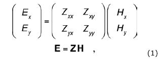
which is a two by two tensor containing the information about electrical resistivity and geometry of the subsurface structures. At each observation site the impedance tensor is estimated as a function of frequency using the natural electromagnetic fields E and H measured at the earth's surface. The ground resistivity distribution as a function of depth is investigated comparing the observed impedances with synthetic data produced by numerical simulations. The observed impedance tensor is usually reduced to an off–diagonal form in order to match with two synthetic impedances produced by 2–D numerical simulations. This is because in a 2–D situation only two impedances are necessary to represent the physical problem: one of them associated with current flow along strike (TE polarization mode) and the other one related with current flow across strike (TM polarization mode). The reduction of four observed tensor elements to a suitable TE and TM responses has been the topic of a large volume of literature (Vozoff, 1991; Ogawa et al., 2001; Ogawa et al., 2002; Ledo, 2006). It is a challenging problem, as it attempts to reduce the 3–D–Earth's response to a 2–D equivalent. A commonly used approach consists of decomposing the full tensor in a regional 2–D off–diagonal form, distorted by local 3–D effects (Bahr, 1988; 1991; Groom and Bailey, 1989; 1991). This method has proved very useful in practice whenever the assumption that any 3–D heterogeneity can be considered as local geological noise perturbing a regional 2–D structure.

Other approaches make no assumptions about the earth's dimensionality. They recognize that the full tensor completely describes the underground response, and uses mathematical transformations in order to find more useful or simpler representations of the response function (Eggers, 1982; Yee and Paulson, 1987; Romo et al., 2005). These transformation methods preserve all the information contained in the original tensor, i.e., it is always possible to retrieve the original tensor elements by means of an inverse transformation.

In this work we used the transformation proposed by Romo et al. (2005),

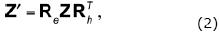
where R_e and R_hare complex operators producing rotation and phase shifts in the electric and magnetic vectors. This transformation yields a couple of impedances: the so–called series and parallel impedances, as well as two additional complex angular functions related with the geometry of the subsurface anomalies,

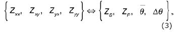
The series and parallel (s–p) impedances Z_S and Z_P contain complementary information, in a similar way as traditional TE and TM modes complement each other. The series impedance is more sensitive to galvanic effects while the parallel impedance is more affected by inductive effects (Romo et al., 2005).

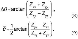
The angular functions Δθ and provide additional information about dimensionality and structural strike. The real part of the angular difference Δθ is a measure of the tensor skew, a quantity commonly used in magnetotellurics as an indicator of three–dimensionality. On the other hand, the real part of the angular average reduces to the impedance strike, which is an estimate of the structural azimuth.

Following Romo et al. (2005), s–p impedances Z_S and Z_P , can be calculated from the four components of the impedance tensor by

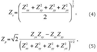
where Z_S and Z_P are frequency dependent complex variables that can be represented by the apparent resistivity and phase curves

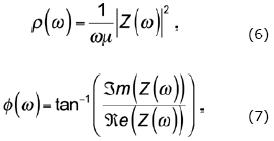
where μ is the free–space magnetic permeability and ω is the angular frequency.

The angular difference Δθ and the angular average are defined by

In summary, the s–p transformation uses the information contained in the full impedance tensor to provide a couple of rotation–invariant responses, sensitive to galvanic and inductive effects, which are useful to constrain multidimensional inversion of MT. In this work we use this approach and the results are compared with those obtained using the tensor decomposition method proposed by Groom and Bailey (1989).

The Groom–Bailey method assumes that the observed impedance tensor is composed by a regional 2–D tensor distorted by 3–D local effects, represented by

R is a rotation matrix and T and S are distortion tensors, named twist and shear, containing the real elements τ, and s. There are seven real parameters to estimate in equation (10): τ, s, and the 2–D complex impedance elements Z_a and Z_b. We estimate this parameters using the optimization approach by Chave and Smith (1994). The goodness of the estimations is tested using a normalized misfit between observed and predicted impedance elements.

MT Data

Temporal variations of the natural electromagnetic fields were registered at 17 sites along the 45–km profile shown in Figure 2, using a 10–channel MT data acquisition system (EMI, Inc.). Most of the time we registered two sites simultaneously so as to use the remote reference estimation technique. At each site, the impedance tensor response was estimated in a frequency band from 0.001 to 100 Hz, using the robust estimation algorithm by Chave et al. (1987).

Dimensionality analysis

3–D effects

We use the real part of Δθ as a measure of the impedance skew, which is a commonly used indicator of three–dimensionality (Swift, 1967). Angular values larger than ±15º (skew > 0.3) are usually indicative of three dimensional effects. Figure 3a shows that 71% of the values estimated in all the sites for the whole frequency range are within ±15º, indicating that 3–D effects are not significant in most of the sites. Another 3–D indicator is the normalized misfit between the observed impedance and the estimation obtained by Groom–Bailey's decomposition method. A normalized misfit larger that 1.0 is indicative that a 2–D regional model is not an acceptable hypothesis. Figure 3b shows the frequency variation of the normalized misfit for all the sites. In most of the sites the misfit is larger than 1.0 for the high frequencies and reduces to values close to 1.0 as period increases, indicating that a regional 2–D model distorted by shallower 3–D heterogeneities may be a reasonable assumption. In some of the sites located in the eastern part of the profile (7, 8, 11, and 16), the misfit ranges from 10 to 100 at the longer periods, indicating a breakdown of the 2–D hypothesis.

Impedance strike

Romo et al. (2005) show that the real part of , in equation 9, is no other than Swift's rotation angle or "impedance strike", which is a good indicator of structural strike, provided that the geometry is close to a 2–D situation (Swift, 1967). The statistics of this parameter is shown as rose diagrams in Figure 4, the whole frequency band was separated into two windows: 0.01<T<1 s in gray color and 1<T<1000 s in black. Notice that the 90º ambiguity inherent in the estimation is not represented in the rose diagrams. In most of the sites the azimuth estimated in both frequency bands are relatively consistent, exceptions are sites 15, 13, 5 and 16, where the change of azimuth with frequency may indicate a change of the structural strike with depth. The low–frequency band has modes close to 320º and/or 40º degrees in most of the sites, but in sites 2, 3, 7, 8 and 17 azimuth values point toward north. As shown in Figure 4, 300º to 350º azimuths are consistent with the strike of the main active faults in the area. Figure 5 shows that the Groom–Bailey's decomposition method produced azimuth estimates with rather more dispersion but in good agreement with our estimations, suggesting that modeling our profile with a 2–D structure is probably safe.

Induction vectors

Induction vectors estimated from the vertical magnetic field (Vozoff, 1991) are also indicative of the structural geometry. In the high–frequency band vertical magnetic field has usually low amplitude and is produced by near–surface lateral heterogeneities. On the other hand, at low frequencies it depends on regional structures. The real part of the induction vectors is commonly used with a sign convention that yields to arrows that point toward conductors and away from resistive features. The induction arrows shown in Figure 6 are very consistent, indicating a conductive anomaly toward SW from San Miguel Fault. The Ojos Negros fault located in–between sites 13 and 14 is also shown as related to a conductive feature. Notice that the number of estimates is not the same in all the sites, this is because we used only high quality estimates with coherency values larger than 0.7.

Static shift estimation

In order to estimate the shift factor in the apparent resistivity curves caused by galvanic effects of shallow heterogeneities, we used a stepwise approach similar to one proposed by Wu et al. (1993) and Ogawa et al. (2002). The first step was to use 2–D inversion to fit only the phase data. The resulting model response was then utilized to estimate the shift factor for the observed "series" (or pseudo–TM) apparent resistivity. In the second step we inverted the apparent resistivity series and phase data as well as the parallel phase (or pseudo–TE) to estimate the shift factor for the parallel apparent resistivity curve. The corrected apparent resistivity curves and the corresponding phases were then inverted simultaneously, as described in the following section.

 

2–D resistivity models

S–P inversion

We used an adapted version of the Gauss–Newton inversion algorithm, originally coded by Rodi and Mackie (2001) modified to include the partial derivatives matrix representing the change of our s–p responses with regards to changes in the model resistivity. The iterative algorithm minimizes the misfit between observed data and model response in the least square sense. At the same time, the roughness of the model is constrained by minimizing the cell resistivity variation. The tradeoff between data misfit and model roughness is controlled by the so–called regularization parameter τ.

Both, series and parallel impedances were simultaneously inverted to produce a resistivity model in a cross–section along the MT profile data. We start from a 10 Ohm–m homogeneous half–space, and look for a resistivity distribution considering a trade–off between data misfit and model smoothness. Excessively smooth models have large data misfits, whereas reducing too much the data misfit could result in unacceptably rougher models. We explore the solution space using different values for the regularization parameter. The best or optimal model was found using the L curve criteria (Farquharson and Oldenburg, 2004), i.e., the model with the best balance between data misfit and model roughness.

Figure 7a shows the best model obtained with a regularization factor τ = 30. This figure displays only the area of interest, as the model extends laterally and with depth by several tens of kilometers in order to avoid numerical effects at the edges. The bar graph at the top of the model shows the misfit obtained at every site. It ranges from 2 to 8 standard deviations (sd), i.e. 10% to 40%, given a noise floor of 5% for apparent resistivity and 2.5 degrees for phase data. After 400 iterations the total misfit, estimated considering the whole data set, was of 22.9% (~ 4.6 sd). Figure 8 compares, in a site by site basis, the observed curves (symbols) with calculated responses produced by our model (continuous line). We show every other site along the line, this includes one of the better fitted data (sites 15 and 7) as well as one of the worse fitted (site 17). The rms values are calculated including the two apparent resistivity curves as well as the two phase curves. It is manifest that both, apparent resistivity and phase are indeed reproduced by the model at most of the sites, in the whole period range. In general, the obtained misfits allow concluding that the resistivity model shown in Figure 7a plausibly explains the MT observations along the profile.

The most striking feature in the model is the high conductivity anomaly located at depth in the western side. This zone has a resistivity as low as 1 Ohm–m, its top is 10–km deep beneath sites 13 to 03 and is dipping eastward to ~ 25 km deep beneath sites 07 to 11. East of site 04 the model shows a high resistivity anomaly (~10,000 Ohm–m), extending practically from the surface down to 20 km. There are small low resistivity zones at shallow depths (1 to 2 km) located beneath sites 12, 06, and 16, respectively. In the eastern end of the model, beneath site 17, there is a low resistivity zone at a depth of 5 km that appears to extend vertically downward. As this zone is in the extreme of the profile, it is not properly constrained by our measurements, thus it will not be included in the discussion.

Conventional TE–TM inversion

Although the aim of this work is not a comparison between distinct approaches for the interpretation of magnetotelluric data, it is worthwhile to show the resistivity model resulting from a more conventional approach, like the Groom–Bailey (GB) decomposition method. The GB parameters in equation (10) were first estimated with no constrictions, the rotation angle estimated in this way is shown in Figure 5. Then, we estimate the impedances constraining the rotation angle to an azimuth of 324º in all the sites, in agreement with the strike of the main structures, which is nearly perpendicular to the profile direction.

The GB estimated impedances were inverted using the original Gauss–Newton code written by Rodi and Makie (2001) for TE–TM 2–D inversion. We used the same model discretization than the one used for the s–p model and the same number of iterations. The model space was searched with different regularization factors; the best tradeoff between data fit and model roughness was obtained for τ = 50 resulting in the resistivity model shown in Figure 7b. In this case the total rms was 33.4%, comparatively higher than the obtained for the s–p model. It should be mentioned that with this data set we can not achieve rms values better than 33%, even using lower regularization factors which emphasize the data fit at the expense of model roughness. This suggests that s–p curves are easier to fit than TE–TM curves, probably because the s–p sensitivity functions take into account wider regions of the subsurface, so that smoother models produce lower misfits. The s–p curves are also a sort of average of the four tensor elements, while the TE–TM curves are, in the 2–D case, extreme values of the off–diagonal, so that higher resistivity contrasts are needed in the model to reduce TE–TM –curves misfit.

A comparison between observed and calculated TE–TM curves is shown in Figure 9. The best fit was obtained in site 05 (3.3 sd) while the worst was for site 09 (13.0 sd). Again, the model response largely reproduces the observations in most of the sites and for the whole frequency range. In conclusion, the model in Figure 7b provides essentially the same subsurface information than the obtained with the s–p data, i.e. a deep conducive anomaly beneath sites 13 to 03, certainly not as extended and with a NE dipping angle not as evident as in the s–p model.

Seismicity data

Micro–seismic activity was registered in the area using 16–20 digital stations deployed in arrays purposely designed to register local activity (Frez et al., 2000). The seismic stations consisted of Reftek 72A–07 seismographs equipped with short–period Mark L–22 three–component seismometers. Thousands of events (0.2 < M < 4.0) were registered during two separate recording periods of one–month each. Estimates of the hypocenter location were carried out for about 400 events, each one registered in a minimum of six stations, and using only stations at epicentral distances shorter than the estimated focal depths. Maximum uncertainties of about 1 km were achieved for 90% of the cases and never exceed 1.5 km; 80% of the locations have origin–time errors less than 0.07 s (Frez et al., 2000). There is not an evident correlation between magnitude and depth, probably because magnitudes registered in this period of time were too small.

Figure 10a shows the epicenters together with some of the faults mapped in the region. The red dots are events located within a 10 km–wide band along the MT profile; black triangles represent the MT observation sites. The epicenters are broadly distributed in a region between San Miguel and Ojos Negros – Tres Hermanas faults; vertically, most of the events accumulate at a depth of 14–15 km, with a secondary shallow group around 4–5 km, as shown in Figure 10b. The hypocenters were calculated using a layered velocity model chosen to minimize the residual arrival times of local events (Frez et al., 2000). A sensitivity test showed that the hypocenters are not sensitive to velocity changes at depths greater than 10 km, as expected because of the local nature of the selected events.

Fault–plane solutions estimated by Frez et al. (2000) for 50 selected seismic events, showed that most of the focal mechanisms for earthquakes located along the SMF are predominantly strike–slip with a small normal component; curiously, they found that three out of four focal mechanisms determined for events located within the Ojos Negros valley region, are purely normal. After the focal–plane analysis Frez et al. (2000) conclude that the tectonic stress acting in the area has a tensional axis in the E–W direction, with compression axis oriented along the N–S direction, in agreement with the regional stress field producing the NE–SW transform faults along the San Andreas–Gulf of California system. On the other hand, they conclude that the normal mechanisms found within the Ojos Negros valley region do not represent enough evidence to determine the source of such distributed activity.

As discussed in the following section, the resistivity models provide valuable independent information that helps to elucidate the structural behavior at depth of the principal faults in the region.

 

Discussion

Figure 7a shows the hypocenter loci plotted over the resistivity model. Filled circles correspond to those located within a 10–km belt centered along the MT profile, while open circles are events located out of this belt (see figure 10a). A remarkable fact is that most of the seismic activity is located bordering the top of the main conductivity anomaly imaged in the resistivity model. The top of this high conductivity anomaly (< 30 Ohm–m) is dipping eastward with an angle of ~40 degrees. It is quite evident that hypocenters occur in a zone with intermediate resistivity (30 to 300 Ohm–m), clustering in the maximum gradient zone. Similar patterns have been reported by Ogawa et al. (2002) and Ogawa and Honkura (2004). The shape of the conductivity anomaly as well as the spatial attitude of the hypocenters allows us to infer the extension in depth of Ojos Negros fault (ONF), as the listric fault sketched in figure 7a. On the other hand, we associate the San Miguel fault (SMF) with a mid resistivity zone (~300 Ohm–m) as shown in figure 7a.

SMF has taken most of the seismologist attention (Shor and Roberts, 1958; Lomnitz et al., 1970; Reyes et al., 1975; Johnson et al., 1976; Brune et al., 1979; Suárez–Vidal et al., 1991; Doser, 1992; Hirabayashi et al., 1996) because it is known as the most active fault in this region, as well as the source of historical earthquakes. Our results reveal that ONF is also an important structure accommodating normal and strike–slip movement; it seems that this fault is responsible for most of the seismic activity that has been mapped with a broad distribution within the Ojos Negros valley. The spatial distribution of epicenters mapped at the surface can be explained because the dip of the fault–plane decreases with depth, thus projecting a large area at the surface level. Alternatively, San Miguel fault is mainly a strike–slip structure with a more vertical fault–plane, thus explaining some of the epicenter alignments mapped at surface. Both structures are in good agreement with the regional stress field produced by the trans–tensive regime prevalent in the area.

The high resistivity anomalies in the model (>1,000 Ohm–m) are likely associated with dry granitic rocks of the PRB. The highest resistivity is indicative of dry rock conditions, occurring in zones where fresh non–fractured granite exists. As granitic rocks become fractured and wet, their resistivity decreases for several orders of magnitude (Olhoeft, 1981). Thus, the mid resistivity values (30 to 300 Ohm–m) may be reasonably associated with fractured granitic zones particularly because they are also associated with the zones where most of the measured micro–earthquakes are breaking.

The source of the deep high–conductivity anomaly in the foot wall of ONF can be associated to several factors; first and foremost to the presence of fluids trapped in meta–sedimentary pre–batholitic rocks. This interpretation is in agreement with the idea that the strong resistivity contrast observed across the ONF may be related to a compositional contrast between meta–sediments in the footwall and fractured plutonic rocks in the hanging wall of the ONF. Moreover, a large body of literature (Shankland and Ander, 1983; Bailey, 1990; Marquis and Hyndman, 1992), argue that water become trapped just beneath the brittle–ductile transition zone at lower crust, because this zone acts as an impermeable layer precluding the upward migration of fluids produced from dewatering of meta–sediments and/or from digenetic and low grade metamorphic processes (Peacock, 1990). In the studied area the brittle–ductile transition zone is located about 13–15 km deep, as evidenced by the focus distribution shown in Figure 10b, and also supported by other analysis of local and regional earthquake activity (Frez and González, 1991). In addition, listric faults commonly occur where brittle rocks overlie ductile rocks in extensional tectonics like the studied area (Shelton, 1984).

In some cases the presence of fluids has been endorsed by independent geophysical information. Mitsuhata et al. (2001) found, in northeastern Japan, that micro–earthquakes occur just above a highly conductive anomaly in coincidence with the presence of S–wave reflectors. Since the S–wave reflectors are indicative of the presence of fluids, the cause of the high conductivity is interpreted as a fluid–filled zone in a porous media. Moreover, they suggest that when the fluid seeps into the surrounding, less permeable (more resistive) granitic rocks, it increases the pore pressure and may become a trigger of micro–earthquake activity.

An additional factor that could produce an enhancement of conductivity is the presence of graphite, even in very small volume fractions (Duba and Shankland, 1982). Graphite is usually found in cataclastic fault zones or as a product of metamorphic processes, particularly in the case of meta–sediments; it has been shown that if properly interconnected, graphitic minerals could become an important cause of conductivity enhancement. In our case we have both, an active fault zone as well as rocks with an intense history of metamorphism, thus the presence of graphitic minerals may be a reasonable cause for the deep high–conductivity anomaly imaged in our model. We do not discard this possibility; however, the trapped fluids argument seems a more plausible explanation.

As a final point, we think that temperature is not a significant contributor to the conductivity enhancement in the area. In this zone the magmatic accretion events ended about 100 Ma ago, thus the temperature expected at 13–15 km depth is about 400°C, which is also in agreement with the location of the brittle–ductile transition zone determined by the location of hypocenters. This temperature range is by itself an insignificant factor for conductivity enhancement, compared with the fluid content (Olhoeft, 1981). Nevertheless, it probably contributes to an increase of the pore–fluid salinity, and so indirectly may increase the bulk conductivity of the rocks.

 

Conclusions

The electrical conductivity anomalies found in the resistivity models are in very good agreement with the location of seismic focus at depth. Moreover, electrical resistivity and seismic information effectively complement each other to reveal the geometry and deep extension of geological structures mapped at the surface.

The positive results obtained in this work as well as their comparison with more conventional approaches confirm that series and parallel invariant impedances are a convenient set of MT responses to be used with inversion algorithms.

We find that ONF is a listric regional structure responsible of most of the seismic activity that has been mapped as broadly distributed within the Ojos Negros valley. The geometry as well as the large resistivity contrast observed across the ONF fault–plane, suggests a compositional contrast between ductile highly conductive pre–batholitic meta–sediments in the footwall, and more brittle mid–resistivity fractured plutonic rocks in the hanging wall. Surprisingly, the conductivity signature of San Miguel fault, considered the most active fault in the region, is not spectacular. It is shown as a mid–resistivity zone along an almost vertical fault–plane. This is likely because SMF is affecting only highly–resistive granitic rocks; moreover it is a relatively young fault with several separate segments unconnected to each other, thus a fluid flow zone has not been completely developed.

The spatial attitude of hypocenters located in a zone of maximum resistivity gradient at the rim of a highly conductive anomaly suggest that seismic nucleation is likely taking place in partially fractured granite just above the brittle–ductile transition zone, where fluid pressure may be playing a decisive role.

 

Acknowledgments

We greatly appreciate and thank the review and comments by Oscar Campos as well as by an anonymous referee. We are also grateful to Y. Ogawa and U. Weckmann, whose comments helped to improve significantly the original manuscript. We thank the personal of the Applied Geophysics department of CICESE who participated in the field work, as well as the personal of the Seismology department who analyzed the seismic data. We are particularly grateful to our colleagues A. Martín, J. Fletcher and L. Delgado for their valuable comments on the geological significance of our results. This project was partially supported with funds provided by CICESE's Geology, Seismology and Applied Geophysics Departments, as well as CONACYT grants 35–228–T, SEP–2004–C01–45834 and SEP–2004–C01–47922/A–1. We are also grateful to CONACYT for the doctorate scholarship grant to R. Antonio–Carpio.

 

Bibliography

Bahr K., 1988, Interpretation of the magnetotelluric impedance tensor: regional induction and local telluric distortion. J. Geophys., 62, 119–127.         [ Links ]

Bahr K., 1991, Geological noise in magnetotelluric data: A classification of distortion types. Phy. Earth Plan. Int., 66, 24–38.         [ Links ]

Bailey R.C., 1990, Trapping of aqueous fluids in the deep crust. Geophys. Res. Lett., 17, 1129–1132.         [ Links ]

Bedrosian P.A., Unsworth M.J., Egbert G.D. Thumber, C.H., 2004, Geophysical images of the creeping segment of the San Andres fault: implications for the role of crustal fluids in the earthquakes process. Tectonophysics, 385, 137–158.         [ Links ]

Brune J.N., Simons C., Rebollar C., Reyes, A., 1979, Seismicity and faulting in northern Baja California. In: Abbot P.L., Elliot J.W. (Editors), Earthquakes and other perils, San Diego region, San Diego, Ca., 83–100.         [ Links ]

Campos–Gaytán J.R., 2002, Actualización de modelo geohidrológico del acuífero del Valle de Ojos Negros, Baja California. M. Sc. Thesis, CICESE, Ensenada, B.C., 151 p.         [ Links ]

Chave A.D., Smith J.T., 1994, On electric and magnetic galvanic distortion tensor decompositions. J. Geophys. Res., 99, 4669–4682.         [ Links ]

Chave A.D., Thomson D.J., Ander M.E., 1987, On the robust estimation of power spectra, coherences and transfer functions. J. Geophys. Res., 92B, 633–648.         [ Links ]

Doser D.I., 1992, Faulting processes of the 1956 San Miguel, Baja California, earthquake sequence. PAGEOPH, 139, 3–16.         [ Links ]

Duba A. Shankland, T.J., 1982, Free Carbon and Electrical Conductivity in the Earth's Mantle. Geophys. Res. Lett., 9, 1271–1274.         [ Links ]

Eggers D.E., 1982, An eigenstate formulation of the magnetotelluric impedance tensor. Geophys., 47, 1204–1214.         [ Links ]

Farquharson C.G. Oldenburg, D.W., 2004, A comparison of automatic techniques for estimating the regularization parameter in non–linear inverse problems. Geophys. J. Int. 156, 411–425.         [ Links ]

Frez J., González J.J., 1991, Crustal structure and seismotectonics of northern Baja California. In: B. Simoneit and J.P. Dauphin (Editors), The gulf and peninsular province of the Californias. American Association of Petroleum Geologists, Tulsa, Oklahoma, 261–283.         [ Links ]

Frez J., González J.J., Acosta J.G, Nava F.A., Méndez I., Carlos J., García–Arthur R.E., Álvarez M., 2000, A detailed microseismicity study and current stress regime in the Peninsular Ranges of northern Baja California, México: The Ojos Negros region. Bull. Seismol. Soc. Am., 90, 1133–1142.         [ Links ]

Gastil R.G., Phillips R.P., Allison E.C., 1975, Reconnaissance geology of the State of Baja California. Memory 140. Geolog. Soc. Am., 170 pp.         [ Links ]

Glover P.W.J., Vine F.J., 1992, Electrical Conductivity of Carbon Bearing Granulite at Raised Temperatures and Pressures, Nature, 360, 723–725.         [ Links ]

Goto T., Wada Y., Oshiman N., Sumitomo N., 2005, Resistivity structure of a seismic gap along the Atotsugawa Fault, Japan. Phy. Earth Plan. Int., 148, 55–72.         [ Links ]

Gratier J.P., Favreau P., Renard, F., Pili E., 2002, Fluid pressure evolution during the earthquake cycle controlled by fluid flow and pressure solution crack sealing. Earth Plan. Spa., 54, 1139–1146.         [ Links ]

Groom R.W., Bailey R.C., 1989, Decomposition of magnetotelluric impedance tensors in the presence of local three–dimensional galvanic distortion. J. Geophys. Res., 94, 1913–1925.         [ Links ]

Groom R.W., Bailey R.C., 1991, Analytic investigations of the effects of near–surface three–dimensional galvanic scatterers on MT tensor decompositions. Geophysics, 56, 496–518.         [ Links ]

Haberland C., Rietbrock A., Schurr B. Brasse H., 2003, Coincident anomalies of seismic attenuation and electrical resistivity beneath the southern Bolivian Altiplano plateau. Geophys. Res. Lett., 30(18), 19–23.         [ Links ]

Hirabayashi K., Rockwell T.K., Wenousky S.G., Stirling M.W., Suárez–Vidal F., 1996. A neotectonic study of the San Miguel–Vallecitos fault, Baja California, México. Bull. Seis. Soc. Am., 86, 1770–1783.         [ Links ]

Ichiki M., Mishina M., Goto T., Oshiman N., Sumitomo N., Utada H., 1999, Magnetotelluric investigations for the seismically active area in Northern Miyagi Prefecture, northeastern Japan. Earth Plan. Spa., 51, 351–361.         [ Links ]

Johnson S.E., Tate M.C., Fanning C.M., 1999, New geologic mapping and SHRIMP U–Pb zircon data in the Peninsular Ranges batholith, Baja California, México: Evidence for a suture? Geology, 27, 743–746.         [ Links ]

Johnson T.L., Madrid J., Koczynki, T., 1976, A study of microseismicity in northern Baja California, México, Bull. Seismol. Soc. Am., 66(6), 1921–1929.         [ Links ]

Ledo J., 2006, 2–D versus 3–D magnetotelluric data interpretation, Surveys in Geophysics, 27, 111–148.         [ Links ]

Legg M., Wong V. Suárez–Vidal F., 1991, Geologic structure and tectonics of the inner continental borderland of northern Baja California. In: J.P. Dauphin and B. Simoneit (Editors), The gulf and peninsular province of the Californias. American Association of Petroleum Geologists, Tulsa, Oklahoma, 145–177.         [ Links ]

Lomnitz C., Mooser F., Allen C.R., Brune J.N., Thatcher W., 1970, Seismicity and tectonics of the northern Gulf of California region, México: preliminary results. Geofísica Internacional, 10, 37–48.         [ Links ]

Marquis G., Hyndman, R.D., 1992, Geophysical support for aqueous fluids in the deep crust: seismic and electrical relationships. Geophys. J. Int., 110, 91–105.         [ Links ]

Mitsuhata Y., Ogawa Y., Mishina M., Kono T., Yokokura T., Uchida T., 2001, Electromagnetic heterogeneity of the seismogenic region of 1962 M6.5 Northern Miyagi Earthquake, northeastern Japan. Geophys. Res. Lett., 28, 4371–4374.         [ Links ]

Nover G., 2005, Electrical properties of crust and mantle rocks – a review of laboratory measurements and their explanation. Surv. Geophys., 26, 593–651.         [ Links ]

Ogawa Y., 2002, On Two–dimensional modeling of magnetotelluric field data. Surv. Geophys., 23(2–3), 251–273.         [ Links ]

Ogawa Y., Mishina M., Goto T., Satoh H., Oshiman N., Kasaya T., Takahashi Y., Nishitani T., Sakanaka S., Uyeshima M., Takahashi Y., Honkura Y., Matsushima M., 2001, Magnetotelluric imaging of fluids in intraplate earthquake zones, NE Japan back arc. Geophys. Res. Lett., 28, 3741–3744.         [ Links ]

Ogawa Y., Takakura S. Honkura Y., 2002. Resistivity structure across Itoigawa–Shizuoka tectonic line and its implications for concentrated deformation, Earth Plan. Spa., 54, 1115–1120.         [ Links ]

Ogawa Y., Honkura Y., 2004, Mid–crustal electrical conductors and their correlations to seismicity and deformation at Itoigawa–Shizuoka Tectonic Line, Central Japan, Earth Plan. Spa., 56, 1285–1291.         [ Links ]

Olhoeft G., 1981. Electrical Properties of Granite With Implications for the Lower Crust, J. Geophys. Res., 82(B2), 931–936.         [ Links ]

Peacock S.M., 1990, Fluid processes in subduction zones. Science, 248, 239–337.         [ Links ]

Reyes A., Brune J., Barker T., Canales L., Madrid J., Rebollar J., Munguia L., 1975, A microearthquake survey of the San Miguel fault zone, Baja California, México, Geophys. Res. Lett., 2, 56–59.         [ Links ]

Ritter O., Weckmanna U., Vietor T., Haak, V., 2003, A magnetotelluric study of the Damara Belt in Namibia: 1. Regional scale conductivity anomalies, Phys. Earth Plan. Int., 138, 71–90.         [ Links ]

Rodi W., Mackie, R.L., 2001, Nonlinear conjugate gradients algorithm for 2D magnetotelluric inversion, Geophys., 66, 174–187.         [ Links ]

Romo J.M., Gómez–Treviño E., Esparza F.J., 2005, Series and parallel transformations of the magnetotelluric impedance tensor: theory and applications. Phys. Earth Plan. Int., 150, 63–83.         [ Links ]

Sarma S.V.S., Prasanta V., Ptro K., Harinarayana T., Veeraswamy K., Sastry R.S., Sarma M.V.C., 2004, National Geophysical Research Institute, Uppal Road, Hyderabad 500–007, India, A magnetotelluric (MT) study across the Koyna seismic zone, western India: evidence for block structure. Phys. Earth Plan. Int., 142, 23–36.         [ Links ]

Shankland T.J., Ander M.E., 1983, Electrical conductivity, temperatures, and fluids in the lower crust. J. Geophys. Res., 88, 9475–9484.         [ Links ]

Shankland T.J., Duba A., Mathez E.A., Peach, C.L., 1997, Increase of Electrical Conductivity with Pressure as an Indicator of Conduction Through a Solid Phase in Midcrustal Rocks, J. Geophys. Res., 102, 14741–14750.         [ Links ]

Shelton J.W., 1984, Listric normal faults; an illustrated summary. AAPG Bull., 68(7), 801–815.         [ Links ]

Shor, G.G., Roberts E., 1958, San Miguel, Baja California Norte, earthquakes of February, 1956: a field report. Bull. Seis. Soc. Am., 48, 101–116.         [ Links ]

Stock J., Martín–Barajas A., Suárez–Vidal F., Miller M., 1991, Miocene to Holocene Extensional Tectonics and Volcanic Stratigraphy of NE Baja California, Mexico. In: M.J. Walawender and B. Hanan (Editors), Geological excursions in Southern California and Mexico. Annual Meeting Geological Society of America, San Diego, California, 44–67.         [ Links ]

Suárez–Vidal F., Armijo R., Morgan G., Bodin P., Gastil R.G., 1991, Framework of recent and active faulting in northern Baja California. In: J.P. Dauphin and B. Simoneit (Editors), The gulf and peninsular province of the Californias. American Association of Petroleum Geologists, Tulsa, Oklahoma, 285–300.         [ Links ]

Swift C.M., 1967, A magnetotelluric investigation of an electrical conductivity anomaly in the southwestern United States. PhD Thesis, Massachusetts Institute of Technology, 226 p.         [ Links ]

Tank S.B., Honkura Y., Ogawa Y., Matsushima M., Oshiman N., Kemal–Tunçer M. Celik C., Tolak E., Isikara, M., 2005, Magnetotelluric imaging of the fault rupture area of the 1999 Izmit (Turkey) earthquake. Phys. Earth Plan. Int., 150, 213–225.         [ Links ]

Vázquez R., Traslosheros C., Vega M., Vega R., Espinosa J.M., 1991, Evaluación geohidrológica en el noroeste de Baja California, CICESE, Ensenada, Baja California.         [ Links ]

Vozoff, K., 1991, The magnetotelluric method. In: M.N. Nabighian (Editor), Electromagnetic methods in applied geophysics, 2, Application. Soc. Explor. Geophys., 641–711.         [ Links ]

Wu N., Booker J.R., Smith J.T., 1993, Rapid Two–Dimensional inversion of COPROD2 data. J. Geom. Geoelec., 45, 1073–1087.         [ Links ]

Yee E., Paulson K.V., 1987, The canonical decomposition and its relationship to other forms of magnetotelluric impedance tensor analysis. Geophys. J., 61,173–189.         [ Links ]

Zhao D., Tani H., Mishra O.P., 2004, Crustal heterogeneity in the 2000 western Tottori earthquake region: effect of fluids from slab dehydration. Physics of the Earth and Planetary Interiors, 145, 161–177.         [ Links ]

Zhao D., Kanamori H., Negishi H., 1996. Tomography of the source area of the 1995 Kobe earthquake: evidence for fluids at the hypocenter?. Science, 274, 1891–1894.         [ Links ]