Articles

 

Significance tests for the relationship between "El Niño" phenomenon and precipitation in Mexico

 

J. L. Bravo Cabrera*, E. Azpra Romero, V. Zarraluqui Such, C. Gay García and F. Estrada Porrúa

 

Centro de Ciencias de la Atmósfera, Universidad Nacional Autónoma de México, Ciudad Universitaria, Del Coyoacán, 04510, Mexico City, Mexico. ^*Corresponding author: afalcon@cibnor.mx

 

Received: August 13, 2009
Accepted: May 21, 2010

 

Resumen

Describimos el comportamiento estadístico de la significancia de las diferencias en la precipitación en México durante la presencia de "El Niño", "La Niña" o condiciones neutrales. La principal diferencia con otros trabajos similares es el análisis de significancia estadística de las diferencias en la precipitación entre diferentes condiciones del fenómeno El Niño – Oscilación del Sur (ENOS). El análisis se llevó a cabo para la estación húmeda (junio, julio, agosto y septiembre), la estación seca (diciembre, enero y febrero) y para el año completo. Se ajustaron líneas rectas por mínimos cuadrados usando la precipitación como variable dependiente y el valor del Índice Multivariado para el fenómeno ENOS (IME) como variable independiente. Se hicieron también comparaciones de la precipitación entre condiciones de "El Niño", "La Niña" y neutras usando pruebas de Wilcoxon – Mann – Whitney. Los resultados muestran que durante la ocurrencia de "El Niño" la precipitación decrece en la parte sur y se incrementa significativamente en el norte y el noroeste de México. Por el contrario, en condiciones "La Niña", la precipitación se incrementa en el sur y decrece hacia el norte. En la parte central de México las diferencias con respecto a las condiciones neutrales no son significativas. El comportamiento, comparando las estaciones húmeda y seca, es diferente. Durante la época húmeda y con condiciones de "El Niño" la precipitación decrece en el sur y áreas centrales permaneciendo relativamente sin cambios en el norte. Con condiciones "La Niña" y en la estación húmeda la precipitación se incrementa en el sur. Durante la estación seca y en condiciones de "El Niño" la precipitación se incrementa hacia el norte y noroeste mientras que con "La Niña" decrece hacia el sur. El fenómeno ENOS explica en promedio entre 3.7 y 8.9% de la varianza de la precipitación, esto puede deberse a los muchos fenómenos climáticos que la afectan y que lo hacen en una proporción variable y desconocida. Sin embargo hay áreas importantes del país en donde el fenómeno ENOS afecta la precipitación de una manera estadísticamente significativa.

Palabras clave: ENSO, precipitación, significancia estadística, territorio mexicano, variabilidad climática.

 

Abstract

We describe the behavior of the statistical significance of the differences in rainfall in Mexico during the occurrence of "El Niño", "La Niña", or neutral conditions. This analysis, which had not been made before, reveals the areas in which the effect of ENSO is statistically significant. The analyses were carried out for the wet season (June, July, August and September), for the dry season (December, January and February), and for the whole year. Straight lines were fitted using precipitation as the dependent variable and the value of the Multivariate ENSO Index (MEI) as the independent variable. We also compared precipitation between different "El Niño", "La Niña" and neutral conditions using the Wilcoxon – Mann – Whitney test. The results show that during the occurrence of 'El Niño", precipitation decreases in the south and increases significantly in northern and northwestern Mexico. By contrast, in years under "La Niña", rainfall increases in the south and decreases towards the north. In central Mexico differences with respect to neutral conditions are not significant. Comparing the wet and dry seasons, their behavior is somewhat different. During the wet season, and under "El Niño" conditions, the rainfall decreased in the southern and central areas, remaining roughly unchanged in the north. Under "La Niña" conditions and the wet season, the precipitation increased in the south. During the dry season and under "El Niño" conditions, rainfall increases towards north and northwest, while with "La Niña" it decreases southwards. The ENSO phenomenon explains between 3.7 and 8.9% of the variance of the precipitation; this may be due to the many weather phenomena affecting precipitation in varying and unknown proportions. Nevertheless, in some important regions of the country the ENSO phenomenon influences the precipitation in a way that is statistically significant.

Key words: ENSO, precipitation, statistical significance, Mexican territory, climatic variability.

 

Introduction

The climatic El Niño–Southern Oscillation (ENSO) phenomenon has two phases: the warm ("El Niño") and the cold ("La Niña") phases, occurring alternatively. These changes include the modification of the Sea Surface Temperature (SST) for large areas of the Pacific Ocean. The changes in SST modify also the climate in a vast area of the planet (Magaña, 1999; Sheinbaum, 2003). Today,for virtually any part of the world anyone could probably find a teleconnection study that relates fluctuations in surface climate to some "El Niño" index (Englehart and Douglas, 2002); these changes affect ecological systems and human societies, sometimes with catastrophic results.

Certain characteristics of ENSO have led to conflicting views, mostly in regard to the irregular occurrence of the warm and cold phases having a mean duration cycle of 4 years, but including irregular cycles of variable intensity lasting anywhere from 2 to 7 years. Such variations make it difficult to predict cycle occurrence (Philander and Fedorov, 2003).

Quinn et al. (1987) studied the "El Niño" phenomenon and made a qualitative classification of intensity throughout the historical records. Since 1950, quantitative estimates have been made which include, in addition to the temperature of the ocean surface, other important variables related to the phenomenon. One of the quantitative evaluations of the intensity of the phenomenon is usually made using the Multivariate ENSO Index (MEI), which consists of six parameters: the atmospheric pressure at sea level, zonal surface (EW) and meridional (NS) winds, sea surface temperature (SST), air temperature at the surface of the sea, and the fraction of total cloud cover. The value of MEI is the first principal component of the normalized covariance matrix after smoothing using cluster analysis (Wolter, 1987; Wolter and Timlin, 1993; Wolter and Timlin, 1998).

Several authors have studied the effects of ENSO in the Mexican territory: Galindo and Mosiño (1992) found at least five precipitation patterns associated with ENSO events, four of them showing precipitation above normal during ENSO episodes. Reyes and Troncoso (1998) studied the effects of ENSO on tropical cyclones of the Pacific and Atlantic oceans that affect Mexico; they found that in the Atlantic Ocean the development of cyclones decreases during "El Niño" while it does not change in the Pacific Ocean. Minnich et al. (2000) and Reyes and Troncoso (2004) studied the effect of the ENSO signal on precipitation in Baja California, finding that the inter–annual variability of annual and monthly precipitation is strongly linked to ENSO events. Magaña et al. (2003) have estimated, using different databases, the impact of the ENSO phenomenon on rainfall in Mexico, although they did not perform tests of statistical significance on the differences they found. Peralta–Hernández et al. (2008) estimated the behavior of rainfall during the mid–summer drought under "El Niño" conditions in central Mexico. Englehart and Douglas (2002) analyzed precipitation during summer, and regionalized the Mexican territory to study teleconnections with some meteorological parameters, including those related to "El Niño". In all these works the statistical significance of the differences between the ENSO conditions are little addressed. Pavia et al. (2006) used bootstrap methods (Efron and Tibshirani, 1993) for the assignment of arbitrary significance to the effect of the interaction of the Pacific Decadal Oscillation (PDO) and ENSO on Mexico's climate, finding weak but noticeable PDO–ENSO influence on climate. Therefore here we describe the behavior of the statistical significance of the differences in rainfall in Mexico during the presence of "El Niño" or "La Niña", treating aspects not fully considered in the works of Magaña et al. (2003) and Peralta–Hernádez et al. (2008). We employ a different procedure than that used by Pavia et al. (2006) to evaluate the statistical significance of ENSO intensity on climate of Mexican territory. In addition, we illustrate the use of simpler statistical methods than those used in some of these works. We used least–squares procedure to fit straight lines to precipitation vs. MEI variables. The significance of the regression is used to evaluate the significance of the relationship. This method was successfully used by Pavia et al. (2009) to study the annual and seasonal trends of temperature in Mexico; therefore they used time as independent variable and temperature as dependent variable. Pavia et al. (2006) used ENSO and PDO classification of precipitation to evaluate the significance of the relation, we used the intensity of ENSO instead of the PDO values assuming an interaction between PDO and ENSO as mentioned by Schneider and Cornuelle (2005), Newman et al. (2003) and Yeh and Kirtman (2004). The aspects treated here had not been fully considered by other authors, and is useful to understand the influence of the ENSO phenomenon in the above or below–average amount of rainfall during periods dominated by the warm or the cold phases of ENSO.

 

Nature of the data

As mentioned in the previous section we used the Multivariate ENSO Index Series (MEI) as reported by the National Oceanic and Atmospheric Administration (NOAA) on its World Wide Web site. We used this index since it involves 6 parameters associated with the phenomenon. Although there are some other indices such as Southern Oscillation Index (SOI) or the Japan Meteorological Agency (JMAI), they generally show a high correlation with the MEI so that the results obtained herein will not differ significantly from those using other indices.

Precipitation was evaluated using the updated database CLICOM 2006. There are approximately 5,928 weather stations with reports of rainfall since 1930 for the 32 states of the Mexican Republic. The amount of precipitation was evaluated with regard to the monthly arithmetic means of daily precipitation. Seasonal and annual averages were calculated from these monthly means. In general, we used only the months with more than 27 days of observations and selected the stations with at least 40 full years between 1950 and 2006; however, in some central states we used stations with only 35 complete years. The objective of this selection is to eliminate, as far as possible, the bias caused by a non–random sampling due to the lack of data. With this selection we attempted to use the most complete set of stations from the database. Only 349 stations met the mentioned characteristics; their geographical positions are shown in Fig. 1. Notice that the distribution is not uniform and that there are large areas without suitable stations for the purposes of this work, for example in Sinaloa and Baja California.

We examined the database and when observational errors or inconsistencies were detected the station was eliminated. Only reported values were used in this study.

 

Methods

To assess the existence of a relationship between rainfall and ENSO we fit least squares straight lines to the values of precipitation vs. values of MEI. We adjusted 3 lines (wet, dry and entire year) to every station. Thus, we obtained 1,047 fits. We used the corresponding annual mean of daily precipitation, or the seasonal mean of daily precipitation, for the wet (June, July, August and September) or dry (December, January and February) periods as dependent variables, and the annual mean of bimonthly MEI values as independent variable for the entire year (or the means of wet or dry seasons of bimonthly MEI values as independent variable). The MEI values reported by NOAA are bimonthly overlapped, we used the MEI value of month (i–1) and month (i) as if it were the value for month (i) only. We used monthly arithmetic means of daily rainfall to eliminate the effect of the variable number of days of observation in the months. The parameters considered in the regression at each weather station were the regression coefficient, b, which is the slope of the adjusted straight line, and a, the y – intercept (x = 0).

Positive values of b mean increase of precipitation with increases of MEI, negative values mean decrease of precipitation with MEI increase. The variance of the regression coefficient is given by

Here s² is the mean square of the unexplained x error, the independent variable, the average of the independent variable, and N the number of observations. The regression coefficient value is significantly different from zero if the calculated value is outside the interval

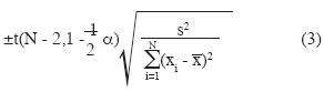
t is the Student parameter with N–2 degrees of freedom and significance a = 0.05 for a two tailed test (Draper and Smith, 1981).

For the use of the Student test the residuals of the regressions must fulfill certain conditions: a) homogeneity of variance, b) independence, and c) normal distribution. We performed the analysis of the residuals and, except in some cases with extreme precipitations, conditions a) and b) were fulfilled. Condition c) is asymptotically fulfilled because we are working with means that, after eliminating their dependence from ENSO, we can consider that the residuals come from the same distribution. Therefore, in virtue of the Central Limit Theorem, their distributions are asymptotically normal. A test on the residuals from the least–squares fittings to the annual data revealed that their distributions are quasi–Gaussian.

To test the classification of Magaña et al. (2003) we used the Wilcoxon–Mann–Whitney test (WMW) to reject the null hypothesis of equality of the distributions of precipitation for the cases of "El Niño", "La Niña", or neutral conditions, which is a procedure free from distribution. The usual two–sample situation is one in which the experimenter has obtained two samples from possibly different populations and wishes to use a statistical test to see if the null hypothesis that the two populations are identical can be rejected. That is, the experimenter wishes to detect differences between the two populations on the basis of random samples from the populations. An intuitive approach to the two sample problem is to combine the two samples into a single ordered sample and then assign ranks to the sample values from the smallest to the largest values, without regard to the population from which the sample came from. Then the statistic test might be the sum of the ranks assigned to those values from one of the populations. If the sum is too small (or too large), there is some indication that the values from that population tend to be smaller (or larger, as the case may be) than the values from the other population. Hence, the null hypothesis of no differences between populations may be rejected if the ranks associated with one sample tend to be larger than those of the other sample.

We used the normal approximation for large samples for the WMW test when there are ties in the data. The statistic test is

where is the sum of the ranks assigned to population 1, n and m are the sizes of samples 1 and 2 respectively, N is the size of both merged samples refers to the sum of the squares of all N of the ranks or averages ranks actually used in both samples when there are ties. This statistic is normal standard distributed (Conover, 1980).

 

Results

The stations were classified according to the sign of the regression coefficient. The results are shown in Fig. 2. The red triangles represent the positive regression coefficients, and the blue diamonds represent the negative regression coefficients. The full signs represent the statistically significant stations. During the years of 'El Niño" the precipitation increases in the north and northwest, mainly in Baja California. In the central part of the country the situation is unclear due to the presence of positive and negative values. In Veracruz, Chiapas, Oaxaca and Guerrero precipitation decreases with "El Niño", and in the Yucatan Peninsula the precipitation increases. Because these results were obtained from the slopes of the straight lines, the trends in precipitation are reversed opposite during "La Niña" in the entioned sites. Statistically significant (p < 0.05) positive values are encountered in Baja California and in the northwest of Mexico, negative values in Veracruz, Hidalgo, Oaxaca and Chiapas. The highest explained variance (R²) was 34.2 % in the Valle de Las Palmas, Tecate (Baja California), while the explained variance throughout the country was only 3.7 %. This agrees with Pavia and Badan (1998) who found a remarkable correlation between the total annual rainfall at Ensenada (Baja California) and the annual signal of the Southern Oscillation Index; and also with Minnich et al. (2000), who reported a strong ENS O signal in Baja California with the increase of rainfall during the warm phase of ENSO.

Considering the wet and dry seasons separately, the geographical distribution of the regression coefficient is somewhat different. The distributions and their statistical significance are shown in Figs. 3a and 3b. During the wet season almost all stations show a negative correlation coefficient, which means a decrease in rainfall during "El Niño" conditions. This result does not agree with the results of Peralta–Hernandez et al. (2008), probably because these authors considered only the mid–summer drought; however, it is in agreement with the fact that only few stations shown statistical significant differences. There are some stations with positive values in central Mexico, and there are also positive values at Chihuahua and Baja California (Minnich et al., 2000). Negative values are statistically significant in central and southern Mexico. This means that in conditions of "El Niño", precipitation decreases during the wet season in most part of the Mexican territory, the significant values occurring in the south. During the wet season the largest explained variance was 32.7 % at Ostuta, Santo Domingo Zanatepec (Oaxaca), and the average explained variance was 5.6 %.

For the dry season almost all stations have a positive correlation coefficient (except in parts of Veracruz, Tabasco and Chiapas), indicating an increase in rainfall with "El Niño" conditions. There are statistically significant regressions throughout all of the country. During the dry season the largest explained variance was 30.2 % in El Oregano, Hermosillo (Sonora), and the average explained variance was 8.9 %. This is in agreement with Reyes and Troncoso (2004) who studied the multidecadal variation of winter rainfall in northwestern Baja California, and signals of SOI and the Pacific Decadal Oscillation. The proportion of winter precipitation with respect to that in summer is shown in Fig. 3c. In Chiapas, Oaxaca, Guerrero, and Jalisco precipitation occurs mainly during summer, and is distributed during the summer and winter in Baja California and Tabasco. In Baja California rainfall occurs in winter, as mentioned by Mosiño and Garcia (1974) and Minnich et al. (2000).

As had been stated before, the significances of the differences from the Magaña et al. (2003) procedure were evaluated using the WMW test, which compares the precipitation between the neutral ENSO and "El Niño" conditions, and neutral with "La Niña" conditions. These tests were performed for the dry and wet seasons. The WMW test compares the equality of the distributions of two samples; thus, in this case there are 4 possible tests: "El Niño" vs. neutral, "La Niña" vs. neutral, and for dry and wet seasons. Following Magaña et al. (2003), the selection criterion was as described below:

For dry seasons and "La Niña" conditions the winters of the years 1964–65, 70–71, 73–74, 75–76, 88–89 and 98–99 were chosen. For the wet season and "La Niña" conditions the summers of the years 64, 70, 73, 75, 88 and 98 were chosen. For the dry seasons and "El Niño" conditions the winters of years 65–66, 72–73, 82–83, 86–87, 91–92 and 97–98 were chosen. And finally, for the wet seasons and "El Niño" conditions 65, 72, 82, 86, 91 and 97 summers were chosen.

The weather stations that are statistically significant for the test are shown in the Figs. 4a to 4d (4b, 4c). Notice that precipitation under "El Niño" and the wet season decreases in almost the whole country. The northwestward precipitation increases, but the weather stations are only statistically significant in the south: on the Pacific coast, and in part of the states of Veracruz, Puebla and Hidalgo.

For "El Niño" and the dry season the precipitation increases in the north and north–central areas. In the south–central and southern parts the results are not clear. At some regions such as the north of Veracruz and central Mexico it diminishes, and in Yucatan and Tehuantepec Gulf the trend is not clear. Only in the north and northwest of the country are the values significant.

For "La Niña" and the wet season the precipitation increases in most parts of the country except in Veracruz and the Yucatan peninsula. The few statistically significant weather stations were located in Jalisco, Puebla and Chiapas.

For "La Niña" and the dry season the precipitation diminishes in almost all of the country, with the exception of some regions in Veracruz, Tehuantepec Gulf, Chiapas and Yucatan. Weather stations with significant values are found in central Mexico, where as we mentioned, the precipitation diminishes.

Tables I, II and III in the appendix, show the principal relationships between the ENSO phenomenon and the rainfall in Mexico.

Figs. 5a, 5b and 5c show the average annual precipitation for the whole year and the wet and dry seasons when the value of the MEI is zero, that is, neutral ENSO conditions. These are the values of the intercept of the linear regression for each weather station. These charts show the arid regions in the north and center, and wetlands in the coastal areas, mainly in the south.

Table IV shows the number of stations with significant statistical values, no significant statistical values and their corresponding percentages.

 

Conclusions

Different statistical tests gave different results because they use different data sets. Regression uses all MEI and precipitation values, while WMW test uses only the order statistics of the data for the selected periods. The regression method gave more weather stations with significant results than the WMW test, and grouping into wet and dry seasons yielded more significant results than the whole year, in agreement with the known fact that "El Niño" produces different effects according to the season of the year.

The fitting of a line to the station data allows the evaluation of the explained variance in precipitation using MEI as independent variable. The explained variance of the average of the daily rainfall by ENSO for the whole country varies between 3.7 and 8.9 %. The maximum of the explained variance in some places was between 30.2 and 34.2% corresponding to the northwest at El Oregano (Sonora) and Valle de Las Palmas (Baja California) or 32.7 % at Ostuta (Oaxaca) at the south of the Mexican territory.

Tables I, II and III from the appendix, show the principal relationships between the ENSO phenomenon and the rainfall in Mexico.

The ENSO phenomenon explains little variance of the precipitation. Variability in precipitation is due to several factors that contribute in different proportions, including the presence and intensity of the monsoon in Mexico, the position of the jet stream, and the frequency and intensity of hurricanes; thus, the detection of the response of the precipitation to a specific cause is very difficult to isolate and evaluate. This variety of effects is an important source of dispersion in the values of the average precipitation, another cause being the inevitable presence of human and instrumental errors in meteorological observations. Nevertheless, in some regions of the country the ENSO phenomenon influences the precipitation in a way that is statistically significant.

 

Acknowledgement

We thank M. en G. Lourdes Godinez for the construction of the figures, Dr. Juan Manuel Espindola for his valuable suggestions and help in correcting the paper, as well as Dra. Shannon E. Kobs and Mr. Enrique Bravo for the final reading of the work.

 

Bibliography

Conover, W., J., 1980. Practical nonparametric statistics, John Wiley & Sons Inc. 215–228.         [ Links ]

Draper, N. R. and H. Smith, 1981. Applied regression Analysis. John Wiley & Sons. 8–25.         [ Links ]

Efron, B. and R. J. Tibshirani, 1993. An Introduction to the Bootstrap. Chapman and Hall, New York.         [ Links ]

Englehart, P. J. and A. V. Douglas, 2002. México's summer rainfall patterns: An analysis of regional modes and changes in their teleconnectivity. Atmós. 15, 147–164.         [ Links ]

Galindo I. and P. A. Mosiño, 1992. Precipitation patters in Mexico associated with El Niño/Southern Oscillation (ENSO). Paleo–ENSO. Records Int. Symp. Lima, Peru, 111–115.         [ Links ]

Magaña, V., 1999. Los impactos de El Niño en México. Dirección General de Protección Civil, Secretaría de Gobernación, México, 229 pp.         [ Links ]

Magaña, V. O., J. L. Vázquez, J. L. Pérez and J. B. Pérez, 2003. Impact of El Niño on precipitation in Mexico. Geofis. Int., 42, 313–330.         [ Links ]

Minnich, R. A., E. Franco and R. J. Dezzani, 2000. The El Niño/Sothern Oscillation and Precipitation Variability in Baja California, Mexico. Atmos., 13, pp. 1–20.         [ Links ]

Mosiño, P. A. and E. García, 1974. The climate of Mexico. World Survey of Climatology. Climates of North America. R. A. Bryson and F. K. Hare (editors). London: Elsevier 11, 345–404.         [ Links ]

Newman, M., G. P. Compo, and M. A. Alexander, 2003. ENSO–forced variability of the Pacific Decadal Oscillation. J. Climate,16, 3853–3857.         [ Links ]

NOAA World Wide Web site: http://www.cdc.noaa.gov/people/klaus.wolter/MEI/table.html        [ Links ]

Pavía, E. G., and A. Badan, 1998. ENSO modulates rainfall in the Mediterranean Californias, Geophys. Res. Lett., 25, 20, 3855–3858.         [ Links ]

Pavia, E. G., F. Graef and J. Reyes, 2006. PDO–ENSO Effects in the climate of Mexico, Journal of Climate, 19, 6433–6438.         [ Links ]

Pavia, E. G., F. Graef and J. Reyes, 2009. Annual and seasonal surface air temperature trends in Mexico, Int. J.Climatol, 29, 1324–1329.         [ Links ]

Peralta–Hernández, A. R., L. R. Barba–Martínez, V. O. Magaña–Rueda, A. D. Matthias and J. J. Luna–Ruíz, 2008. Temporal and spatial behavior of temperature and precipitation during the canícula (midsummer drought) under El Niño conditions in central México. Atmos., 21, 265–280.         [ Links ]

Philander, S. G. and A. Fedorov, 2003. Is El Niño sporadic or Cyclic?. Annu. Rev. Earth Planet. Sci. 31, 579–574.         [ Links ]

Quinn, W. H., V. T. Neal and S. E. Antunez de Mayolo, 1987. El Niño occurrences over the past four and a half centuries. J. Geophys. Res. 92, 14449–14461.         [ Links ]

Reyes, S. and R. Troncoso, 1998. El impacto del fenómeno El Niño – Oscilación del Sur en la generación de ciclones tropicales alrededor de México. Rev. Cienc. Mar, 5, 3–22.         [ Links ]

Reyes, S. and R. Troncoso, 2004. Modulación multi decenal de la lluvia en el Noroeste de Baja California, Rev. Cienc. Mar. 30,99–108.         [ Links ]

Schneider, N. and B. D. Cornuelle, 2005. The forcing of the PDO. J. Climate, 18, 4355–1373.         [ Links ]

Sheinbaum, J. 2003. Current theories on El Niño southern oscillation: A review. Geofis. Int. 42, 297–305.         [ Links ]

Wolter, K., 1987. The Southern Oscillation in surface circulation and climate over the tropical Atlantic, Eastern Pacific, and Indian Oceans as captured by cluster analysis. J. Climate Appl. Meteor. 26, 540–558.         [ Links ]

Wolter, K. and M. S. Timlin, 1993. Monitoring ENSO in COADS with a seasonally adjusted principal component index. Proc. of the 17th Climate Diagnostics Workshop, Norman, OK, NOAA/N MC/CAC, NSSL, Oklahoma Clim. Survey, CIMMS and the School of Meteor., Univ. of Oklahoma, 52–57.         [ Links ]

Wolter, K. and M.S. Timlin, 1998. Measuring the strength of ENSO: how does 1997/98 rank? Weather, 53, 315–324.         [ Links ]

Yeh, S.–W., and B. Kirtman, 2004. The North Pacific Oscillation–ENSO andinternal atmospheric variability. Geophys. Res. Lett., 31, L13206, doi:10.1029/ 2004GL019983.         [ Links ]