Articles

 

Interpretation of Las Salinas sedimentary basin–Argentina, based on integration of geological and geophysical data

 

E. A. Azeglio¹*, M. E. Gimenez² and A. Introcaso³

 

¹ Instituto Geofísico Sismológico Volponi, Facultad de Ciencias Exactas, Físicas y Naturales, Universidad Nacional de San Juan, Av. J. I. de la Roza y Meglioli S/N, Rivadavia, San Juan, 5400. Instituto de Investigaciones Tecnológicas – Ministerio de Producción y Desarrollo Económico, Gobierno de San Juan. Tucumán 1927 (N), Capital, San Juan, 5400. ^*Corresponding author: estudioazeglio@yahoo.com.ar

² CONICET, Instituto Geofísico Sismológico Fernando Volponi, Facultad de Ciencias Exactas, Físicas y Naturales, Universidad Nacional de San Juan. Av. J. I. de la Roza y Meglioli S/N, Rivadavia, San Juan, Argentina, 5400.

³ CONICET, Instituto de Física Rosario. Facultad de Ciencias Exactas, Ingeniería y Agrimensura. Av. Peregrini 250 Rosario, 2000.

 

Received: July 1, 2009
Accepted: September 10, 2010

 

Resumen

La cuenca sedimentaria de las Salinas está ubicada en aproximadamente 3 Iº de latitud sur y 67° de longitud oeste de Argentina, tiene algo más de 100 km de largo, unos 50 km de ancho y una altitud media de 500 m sobre el n.m.m. La cuenca, de rumbo NNW–SSE, está encajada entre las Sierras de la Huerta, las Guayaguas y las Quijadas al oeste, y las Sierras de Chepes, Ulapes y San Luis al este. Ella abarca un área aproximada de 5,700 km² con una profundidad media de 5 km que crece hacia el norte. Por el sur está separada de la cuenca de Beazley por la dorsal de San Pedro.

Nuevos datos de gravedad y valores de archivo, datos de densidades (de pozo) y reinterpretaciones sísmicas permitieron obtener un modelo integrado que involucra: a) un basamento técnico a profundidad de 3.5 km obtenido a partir de reinterpretaciones sísmicas; b) un basamento cristalino con una profundidad media de 5 km obtenido desde datos de gravedad invertidos; c) un fallamiento perimetral e interno que alcanza los 11 km de profundidad que insinúa una disposición lístrica profunda en un estilo de piel gruesa, obtenido desde reinterpretaciones sísmicas 2D, desde técnicas espectrales y desde los alineamientos obtenidos a partir de las soluciones gravimétricas de Euler; d) una sucesión de densidades extraídas desde datos de pozo que permitieron realizar una inversión desde las anomalías de Bouguer operando con densidad variable; y e) un sistemas de tres anticlinales asimétricos cortado por tres sistemas de fallas inversas. f) Una estructura regional que evidencia y dimensiona el esquema compresivo al que ha sido sometida la región. Esperamos que nuestro modelo integrado, con excelente definición, contribuya a la búsqueda de estructuras geológicas de interés económico.

Palabras clave: Modelo geológico–geofísico integrado, reinterpretación sísmica, inversión gravimétrica 3D, cuenca de Las Salinas, Argentina.

 

Abstract

Las Salinas sedimentary basin is located at 31° S and 67° W approximately, in the central–western part of Argentina. Its dimensions are 100 km long, about 50 km wide, plus an average altitude of 500 m above sea level. The basin is situated among the mountain ranges of De la Huerta, Guayaguas and Las Quijadas to the west, and the ranges of Chepes, Ulapes and San Luis to the east, with a NW–SE orientation. Its surface is approximately 5,700 km² with an average depth of 5 km increasing in a northerly direction. The southern part of the basin is separated from the Beazley basin by the buried San Pedro ridge.

New gravimetric information and archive file data, density data (from wells) and seismic reinterpretation allowed us to obtain an integrated model, which involved: a) seismic basement situated at a depth of 3.5 km obtained from seismic reinterpretation; b) crystalline basement with an average depth of 5 km obtained from inverted gravimetric data; c) perimeter and internal faults system reaching 11 km in depth suggesting a listric type disposition in depth, thick–skinned type, obtained from 2–D seismic reinterpretation, spectral analysis technique and alignments obtained from Euler's technique; d) succession of density data extracted from wells allowing us to perform a gravimetric inversion from Bouguer's anomalies operating with variable density; e) a system of three asymmetric breached anticlines crossed by three systems of inverse faults and f) regional structure serving as evidence, permitting us to dimension the compressive framework to which the region has been subjected.

Our purpose is that this well–defined integrated model will contribute to the search for further geological structures of economic interest.

Key words: Geological and geophysical integrated model, seismic reinterpretation, 3D gravimetric inversion, Las Salinas Basin, Argentina.

 

Introduction

Las Salinas basin is located in the northwestern extreme of San Luis province, Argentina extending between the Valle Fertil and De Los Llanos ranges. It borders on the south with the San Pedro Dorsal and continuing up to the north reaching the southern part of La Rioja province (Fig. 1). The basin extends from north to south for approximately 100 km, it is 50 km wide and lies at a mean altitude of 500 m above sea level.

Since the 1980's the region has been an area of noted interest in hydrocarbon prospects, being explored by 2–D seismic reflection studies and drilling in the "Salinas de Mascasin" salt flats (LR.SM.es–1) and "Las Toscas" (SJ. LT.X–1) with the mentioned intentions.

Both drillings documented presence of gas and traces of oil. Seismic studies performed by former state–owned company YPF and other companies in the area, in spite of the low quality of the seismic recordings that hindered its interpretation, showed anticlines with faults, limiting at least four blocks through fractures in length (Fig. 2). The first results interpreted showed that these blocks affect the sedimentary cover, which in the northern extreme, surpasses 3,500 m in thickness. The region shows a shortening due to basin compression that affected the sedimentary cover (Criado Roque et al., 1981; Gardini et al., 2002).

The main structures correspond to a series of asymmetrical anticlines of N–NE disposition, with a short western limb with more inclination associated with inverse fault propagation that dip to the east, thick–skinned type, product of Mesozoic structure inversion (Schmidt et al., 1995; Gardini et al., 1999, 2002, Azeglio et al., 2008). This process is observed in the deep reverse fracturation that elevated Mesozoic and Tertiary rocks at surface level (Criado Roque et al., 1981).

Another structural element considered is the San Pedro buried ridge that constitutes the southern limit of the Las Salinas basin, separating it from the Beazley basin. The San Pedro buried ridge, as a structure, is an active threshold, dating back to the Cretaceous that has controlled sedimentation of the surrounding basins (Criado Roque et al., 1981). It is of W–E direction, formed by two small blocks limited by two faults, one being General Roca and a smaller one, parallel to it and localized to the east.

In the last 3 years we have performed gravimetric measurements in the area under study, with the objective of intensifying the underground knowledge, with the intention of covering the gaps lacking information in the search for geologic structures of interest.

In the present study, we show the results of the integration of the re–interpretation of the existing 2–D seismic lines, the application of different techniques (spectral analysis, Euler solutions, 3–D inversions, 2–D modeling) to the gravimetric file that is enriched with the application of new measurements and the geological knowledge in the area of the Salinas basin.

 

Geologic information

The study of outcrops of the geologic units in the Eastern and Western ranges located in the margins of the Salinas basin (indicated as 4, 5, 6 and 7 in Fig. 1), provides an idea of the stratigraphy that fills the basin and the structures that originated there.

The Guayaguas and Catanal ranges are located in the central–western part of the Salinas basin. They are primarily made up by Mesozoic sediments deposited in basins that originated during the continental extension (Uliana et al., 1989). According to Gardini et al. (1999), this afore– mentioned feature allowed for the generation of different depocenters that contained continental registers deposited mainly during the Triassic and Cretaceous. The Andean compression which followed produced the tectonic inversion of the Mesozoic structures and the present morpho–structural configuration of the western ranges and the surrounding basins.

In the Catantal and Guayaguas smaller ranges the regional extension phenomena seem to be mainly centered in Cretaceous, controlled by dominant faults present in the western margin of the depocenters. The resulting basins were separated by structural heights emerging from the crystalline basement, as seen in the El Gigante range (see Fig. 1) and the positive sectors that today are sub–cropping and only permitted the deposition of the thinner sequences and dynamics (Gardini et al., 1999).

To the east and marking the basin border, upper Cretaceous deposits outcrop, represented basically by the Lagarcito Formation, revealing a broad extension in depth.

The sedimentary column is completed by sequences imprecisely assigned to Tertiary and Quaternary (Gardini etal., 1999; Snyder,1988).

The mentioned rocks outcrop surrounding the Mesozoic sediments, following the brachi–anticline geometry of the main folds. In the western sector, scarce outcrops are generally semi–covered by Quaternary sediments (Gardini et al, 1999).

To the east of the Las Salinas basin lie the Minas and Ulapes ranges (Fig. 1) that constitute a block of crystalline basement of Pre–Carboniferous to Lower Paleozoic age composed mainly by granitoids, with sporadic outcrops of metamorphic rocks, on the continental sediments of Carboniferous, Tertiary and Quaternary are leaning on (Weidmann et al., 1998).

A summary of the existing stratigraphy, sedimentolo–gical and structural information for this area and the well profiles LR.SM.es–1 and SJ.LT.X–1 are summarized in Table 1 and Figs. 2 and 3 respectively.

The stratigraphic names, lithologies, thicknesses and ages were compiled from Bossi (1976), Flores (1979), Criado Roque et al. (1981), Gardiniet al. (2002), Hünicken et al. (1981), Pascual and Bonesio (1981), Schmidt et al. (1995), Snyder (1988), Azeglio et al. (2008) and Eurocan Bermuda (1993).

 

Methods

Seismic data processing

The SEG – Y format files of 2–D seismic line data from the Las Salinas sedimentary basin were also used with YPF oil company information from the Las Toscas (SJ.LT.x–1) and Mascasín (LR–SM.es1) exploration holes.

Due to the inferior quality of the data acquisition, some seismic lines presenting noise high levels were not considered, reinterpreting only lines W–E: 28088, 28087, 28049, 28085, 28093, 28094, 28083, 28095 and N–S: 28092, 28086, 28084, 28090, 28097, 2142B, 2146A, 28108, 28096 and 25117 – 02.

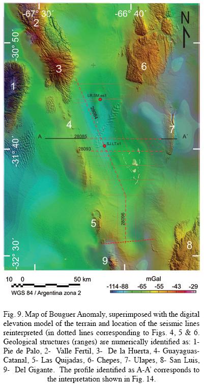
Location of reinterpreted seismic lines is shown in Fig. 9.

The 2–D seismic lines were acquired in the 1980's by YPF with 'VIBROSEIS' recorded at intervals of 6 seconds. The spacing between the stations is 50 m with an offset of 300 m and 1,750 m in 48 channels and symmetric spread obtaining a fold of 24. Nevertheless the data are of inferior quality.

The processing of the seismic lines implemented the Standard Processing Method:

1. Reading of the bands.

2. Bandpass filter (eliminating noise).

3. AGC Filter (drop in amplitude).

4. Balance of the amplitude tracings.

5. Filters F–K (frequency – wave N°).

6. Self–correlation test.

7. Predictive deconvolution.

8. Bandpass filter (elimination of interference–noise residues).

9. Muting velocity (remove air waves).

10. Statistical corrections.

11. Speed analysis using the semblance vs. traveling time & stack speed.

12. Correction of normal move out using the Speed functions.

13. Stacking CDP.

14. Coherence filter.

15. Migration.

For the reinterpretation of the seismic lines (SEG – Y format), the following methodology was applied:

1) Identification and interpretation of a seismic horizon reflectors for each seismic lines.

2)  Analysis of the continuity of the intersection of lines with a 5% margin of error.

3) By relating the intersection of every seismic line a file (in ASCII format) was formed, the 'time horizon'.

4) The procedure was repeated in the same manner for each seismic horizon reflector.

5) Later the stacks velocities transformed into depths based on the DIX Formula (1955).

The data obtained from the Las Toscas well was used in the calibration of seismic horizons (SJ.LT.X1) –(Eurocan Bermuda 1993) – with data from depth/time log, radioactive profile (GR), sonic profile, acoustic impedance, reflection coefficients, synthetic seismic profile and a 40–trace segment of a piece of seismic line 28093 with center in the hole (see Fig. 3). The existing correlation between the stratigraphic horizons found in hole SJ.LT.x–1 and the corresponding seismic horizons in line 28093, are shown in Figs. 3 and 5.

The designation of the ages to the seismic horizon was made by comparing sedimentary and lithological characteristics among outcrops, cores and logs recorded in SJ.LT.x1.

Once the horizons of the profile were identified, this interpretation was extended to all 2–D lines. The identified features were: fault traces and two sedimentary levels on the top of the roof of the seismic basement, which correspond to the top of the Triassic and Cretaceous sediments.

Due to the difficulties of laterally distinguishing the border between Carboniferous and Triassic, we assumed the entire sedimentary unit to be Triassic. This permitted us to draw up an isochronic map (in TWT) of the basement that was later converted to depth through adequate analysis of speed.

A correlation of fault traces interpreted in each seismic section was realized, identifying them in the map of basement through the following identifications F1, F2, F3, F4, F5, F6,.......and F12. Moreover the existence of some very localized fault traces which impeded linking with other lines, were identified by dotted black lines.

Figs. 4, 5, and 6 show three seismic lines to be representative of the area under study.

In Figs. 4, 5, and 6 effect of the compressive stresses to which the region is subjected can be observed, manifesting a complex relation between the two fault systems that surpass the basement, the main fault predominantly N–S and the secondary, to a lesser degree, in a dominant SW–NE direction, both asserting a high dip to the east and south respectively at the surface, insinuating to horizontality in depth. The basin presents an irregular basement, whose geometry is ruled by the described fault systems. It is also observed that Triassic, Cretaceous and even Tertiary strata (San Roque Formation), besides being affected by reverse faulting, present anticline type folds with a short western limb and higher dip, associated with reverse fault propagation to the east.

The structures in Figs. 4, 5, and 6 also show that compressive stress were post –Tertiary and active to present day. Since the fault system is almost projected to the surface and the stratigraphy shows certain parallelism among sediments Triassic to Tertiary periods.

A similar conclusion can be obtained by analyzing the folding in the strata. In the analyzed seismic sections it is observed that Triassic and Cretaceus sediments are in agreement, presenting similar displacements, with values increasing in a southerly direction, with times of 500 ms in line 28085, reaching maximum values of 1,300 ms in line 2195, with a great predominance of 900 ms values.

The reinterpretation of seismic lines in a prevalently north–south direction facilitated the identification of four fault systems that cross the basin in a direction near the perpendicular to its major axis. It is comprised of high angle faults and great displacement, between 500 and 1000 ms, identified in Fig. 6 (representative example) and Fig. 7 as in F9, F10, F11 and F12.

 

Basement seismic modeling

Previous to the basement modeling, a time–to–depth conversion was performed based on the information obtained from the hole recordings and the information obtained from the seismic lines, it was considered a Seismic Datum of 500 m above sea level and a re–emplacement velocity of 2,000 m/s. Sonic data from the hole at a depth of 150 m, corresponds to a sonic recording of 114.4 u.s./f.

The calculation of the instantaneous velocities was:

AV = 1986 + 0.4159 * TWT (AV = Apparent Velocity)

Or with an improved adjustment:

AV = 2065 + 0.2662 * Depth

Where:

AV = Apparent Velocity (Expressed in meters per second)

TWT = Two–Way–Time (Expressed in milliseconds)

DEPTH = Expressed in MetersThis depth is obtained by means of an empirical formula.

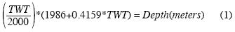
According to (1), the depth of the roof of the basement is calculated at 2,728 m and from the sonic log, the depth of the roof of the basement is located at 2,648 m the difference between the two values is 3%.

The basement modeling was realized by implementing specific software (Z–MAP Plus 2003.13), which allowed us to ponder the depth to top of the basement and the position of the faults found in the seismic profiles, results are shown in Fig. 7. For the interpretation, identification was done as follows: red circles = seismic holes, in black = recognized fault systems and correlated as F1, F2, F3... F12, in a continuous red line = basin border. Numbers 3, 4, 5, 6 and 7 indicate the previously mentioned structures in Fig. 1.

The seismic basement is observed as steep and irregular, governed by a predominant fault system N–S direction, with fault steps of 550 m in the area of line 28085, increasing progressively in a southerly direction reaching values of 1,600 m. These structures are considered products of tectonic inversion that produced major thrust of dominant W–E direction. This compressive stress of N–S direction component provoked the development of a minimum of four release faults marked as F9, F10, F11 y F12 in Fig. 7. The northern fault named F10, divides Las Salinas basin from Marayes basin and the southern fault named F9 defines the southern end of the basin. It is also observed that in the north–eastern sector of the basin, there is a non–outcropping basement marking the east and west borders in an almost perfectly straight manner.

 

Acquisition and processing of gravimetric information

In order to obtain more subsurface information from the area that covers the basin and neighboring ranges, 1,350 new gravimetric determinations and global positioning system (GPS) were also added to the database of the Rosario Physics Institute – Rosario National University and Volponi Seismological – Geophysical Institute –San Juan National University. By applying this new technology, the area was broadly covered in the Las Salinas basin and neighboring areas. All gravimetric data were referred to the International Gravity Standardization Net of 1971 (Morelli, 1974). Geographic positioning was obtained with Geodesic GPS equipment Trimble 5700 model, working in a differential mode with a GPS base located at a distance not exceeding more than 50 km.

The calculation of the gravity anomalies was performed by means of a classic expression (see e.g., Hinze et al., 2005):

Where:

BA: Bouguer anomaly

G_obs: Observed gravity: Linked to the Miguelete Base Station (Buenos Aires Province).

γ₀: Normal gravity at the latitude of the station.

cal: Free Air reduction

cB: Bouguer reduction

ct: Topographic reduction within the Hayford zone, with circular terrain segments (of up to 167 km in diameter, with values of ± 3.5 mGal.

A normal gradient of 0.3086 mGal/m, is contemplated for the reduction of Free Air while a density of σ = 2,67 g/cm³ is assumed for the Bouguer reduction (Hinze, 2003) so that:

Where h: = meters above sea mean level

Later the Bouguer anomaly map was obtained by performing the regularization of the data by applying the Briggs method (1974) of minimum curvature, with a 2.5 x 2.5 km of net gridded.

Figure 8 shows location of the gravimetric stations used in this study.

The quality of the gravimetric reading is sufficiently optimal to make reliable interpretations of the zone under study. Aside from this it is purely expeditive data whose quality diminishes conforming to the spacing increase between stations.

Figure 9 shows the Bouguer anomalies super–imposed on the digital elevation model, observing that the whole map presents negative anomaly values with a notable gradient towards the west, as a consequence of the influence produced by the existence of the Andes root. It is also noteworthy that Las Salinas basin reveals a gravimetric minimum of nearly –80 mGal, with respect to less negative values in both margins, in concordance to neighboring hills.

 

Gravimetric filtering

Since the aim of this study is to emphasize the first kilometers of the crust, it is necessary to separate the gravimetric effects that respond to deep geological structures from superficial effects that respond to shallow ones. In order to do so, distinct filtering techniques were applied to the gravimetric field such as upward continuation performed at different heights (Pacino and Introcaso, 1988) and band pass filters (Blakely, 1995). The map of the Bouguer residual anomaly was obtained from the resulting difference between the observed anomaly (Fig. 9) and the upward continuation extended up 30 km. This result is presented in Fig. 10.

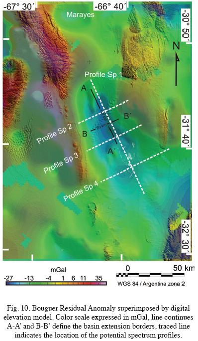
In the Bouguer residual anomaly chart (Fig. 10), the existence of a small, high structural high is clearly observed, it is a deep extension of the De La Huerta range and two split depocenters, one located to the north corresponding to the Mascasin basin and to the south Las Salinas basin. They are both bordered in the west by Valle Fertil–Guayaguas–Catantal ranges and to the east by Chepes and Ulapes ranges. The first approximation, according to the Bouguer residual anomaly (Fig. 10), proposes that Las Salinas basin would be approximately 115 km long and 50 km wide, therefore yielding an estimated surface of 5,750 km².

 

Spectral analysis of the gravimetric results

The spectral method allows us to perform a depth estimation of a source system, from the identification of wave numbers that compose the potential fields produced by the system mentioned (Spector and Grant 1970; Bhattacharya and Leu 1975, 1977; Urrutia Fucugauchi et al., 1999).

The depths of the tops of these bodies are related to the slope logarithm of power spectra as a function of the frequency. The depths represent statistical estimations of the interphases allowing us to evaluate an average structural model (Martinez and Introcaso, 1999; Introcaso, 1999).

In order to evaluate the average depth of the sedimentary units, from the crystalline basement to the topographic surface, four profiles were elaborated, one parallel and three transverse to the major axis of the basin (Fig. 10). The responses manifested in the profiles, are affected by the basement influence, from the basin sedimentary filling and the positive structures of the eastern borders (Chepes– Ulapes system) and west (La Huerta – Guayaguas – Catantal systems).

It is convenient to highlight that the positive structures (either outcropping or not), contaminate the input signal, if the objective is to evaluate the depth of the basement–sediment interface.

The power spectrum that corresponds to the four profiles, is presented in Fig. 11, where the adjustment line and depth, measured in km, is delineated.

The results obtained from profiles for depth of the basement–sediment interphase were: Sp1= 5.3 km, Sp2= 5.49 km, Sp3= 5.18 km, Sp4= 4.08 km.

Basing on interpretations of these results confirms that the structures deepen to the north, as seen in the Bouguer residual anomaly chart, where a negative increase of anomaly values is qualitatively observable; associated with an increase of the sedimentary column thickness in a northwestern direction. This result is consistent with the original information from the seismic holes, where it is known that the top of the Paleozoic sediments in the Mascasin salt flats (located in the northern part of the basin) is deeper than the one in Las Toscas (see Table 1).

The differences in depth values between the seismic hole data and that obtained through specter analysis technique, is because for seismic techniques, the basement is the base of the Carboniferous whereas for the spectral analysis, basement is the contrast surface between the average density of the sedimentary packet with an estimated density of 2.75 g/cm³ presumed to be crystalline basement.

 

Euler deconvolution

Euler's deconvolution technique is frequently used to estimate localization and depth of contrasting density zones in the potential field analysis. This method was presented by Thompson (1982), for 2–D profiles and later by Reid et al. (1990), for gridded data.

Euler's deconvolution is based on the application of Euler's homogeneity equation for a mobile window data for a fixed parameter termed structural index. For each position of the mobile window, a linear system of overestimated equations obtained the position and depth of the sources (Thompson, 1982; Reid et al., 1990; Roy et al., 2000; Mushayandebvu et al., 2004). This technique was applied to the gravimetric gradient, to obtain preliminary estimations of the causative sources for the generation of the observed field. In this process only two parameters can vary. One is the structural index, associated with the geometry of the generating source– represented by a varying number from 0.5 – 2 (Roy et al., 2000). The other is the window width. The window width has to be adapted to the structural dimensions of the target with the goal of obtaining optimal results.

Ideally, signifying for a determined window width, only one type of anomaly should be captured and consequently, fits adequate results (location and depth).

For the particular case of the Las Salinas basin, the best representative results of geometry and depth of its geological structure are obtained with a structural index of 0.7 (Durrheim et al., 1997; Barbosa et al., 1999; Roy et al., 2000; Cooper, 2006) and a window width of 10 km over a 1 X 1 km. grid, considering a 10% margin of error.

The smaller the window, the more emphatic the shallow non–homogeneities will become, usually presenting short wave lengths (Silva et al., 2001). In this way the resolution effectiveness diminishes for the deeper structures and/or those of greater wavelength.

Figure 12 presents the Euler's Standard method application results with the aforementioned parameters. Only the solutions corresponding to the study area are shown. The majority of the solutions are found between 4 and 8 km in depth (yellow, green, and red–colored solutions). Likewise, sketches of a lesser group of solutions from depths less than 4 km (light blue solutions), combined with and in lesser solution amounts reaching 11 km are visualized (blue–colored solutions).

This can be explained because the window width used favors structure identification whose wave lengths are less than 10 km.

The results interpreted from Euler's Deconvolution solutions (Fig. 12) have individualized seven lineaments or a possible fault system numbered as a, b, c, d, e, f, and g. For better linking, the seismic labeling has been retained for those zones where a noticeable coincidence exists between interpreted faults from seismic techniques and lineaments interpreted with Euler's Deconvolution. In faults of N–S direction, especially those identified as a, b, c and g; an appreciable solution migration to the west is seen, as depth increases. This could be explained by a flattening tendency to the east of the fault system, simultaneously with the increase of depth and/or a set of faults in such proximity that, the resolution of Euler's solutions is insufficient to define them conclusively.

The lineament defined by c (Fig. 12), is that which divides the basin in two and presents the least solution dispersion.

Small faults with a N–S tendency identified as d and e are related to the orogenic structure Chepes and Ulapes ranges. Finally the f lineament, defines the southern closure of the basin.

 

Gravimetric inversion model

To estimate the depth to the crystalline basement of the Las Salinas basin, we calculated an inversion of the Bouguer Residual Anomaly (Fig. 10). Gravity modeling requires knowledge of densities of subsurface bodies, which can be approximated by using standard relationships between densities and seismic wave velocities of igneous and metamorphic rocks (Ludwig et al., 1970; Brocher, 2005) or similar velocity–density relationships. Gardner et al. (1974) derive an empirical relationship between density of commonly observed subsurface sedimentary rock and the velocity of propagation of seismic waves through the rocks. We used the available seismic velocity model for the Well SJ.LTx–1 and LR.SM.es–1 (Table 1).

From the sonic log we then obtain the velocity value of sedimentary rocks. We used the results as an input datum in the expression given by Gardner et al. (1974) to obtain the density value for the basin fill.

A GMSYS 3D model software is comprised of a series of one or more layers, defined by grids, overlying a half–space (Parker, 1972). Each layer is assigned density value: topography = 2.67 g/cm³, sedimentary rocks vary with the depth (according to the conversion to depth from sonic log in SJ.LT–x–1 hole) and the basement is assigned a value of 2.75 g/cm³ by extrapolating values obtained from seismologic studies by (Regnier et al. 1994) for the Pie de Palo range and the San Juan Precordillera. GMSYS 3D^® utilizes fast Fourier transform (FFT) calculations to compute the model response. All grids must be expanded in size and filled so they are periodic and eliminate edge effects (Blakely, 1995). In this case, we used 20% for expanded grid, and the grid separation of 2500 m.

When the area has Rugged Topography, care must be taken to ensure the depths to horizons of interest are reported relative to the datum of interest (Cordell, Lindrith, 1985).The topographical surface is the most practical frame of reference for measuring depths to density changes. But inversion of the gravity field is calculated relative to a horizontal plane. In this work, the plane was at 2,200 m above sea level.

The result of gravity inversion of the Bouguer residual anomaly calculated with GMSYS 3D and transformation to depth below the topographic surface is a map of the top of the crystalline basement of the basin are shown in Fig. 13. The black lines and dark red mark the interpretation of a fault system dominating the basin geometry, obtained through seismic techniques and Euler Deconvolution technique. Continuous blue lines identified as I, II and III complete the basin geometric interpretation based on results obtained through the inversion model, observed jointly with Fig. 12.

 

2–D gravimetric interpretation

A 2–D modeling was performed, justifying the Bouguer residual anomaly chart, along an E–W section that coincides to a great extent with seismic line 28085 and covers Ulapes range, to the east, and Guayaguas range, to the west outcrops, see Fig. 9.

In order to execute the modeling, we considered the geological information, seismic line interpretation, depths from spectral power method and lineaments interpreted through the Euler Deconvolution technique. The densities were extracted from sonic log profiles of seismic wells LR.SM.es1 & SJ.LT.x1.

The upper crustal model proposed (Fig. 14), consists of two layers whose densities are an average density of 2.35 gr/cm³ for the sedimentary packet and 2.75 gr/cm³ for the basement. The 2–D gravimetric inversion model was performed through software based on Webring's (1985) technique.

In this model, the consequence of compressive stresses that originated production of reverse faults propagation verging west in a thick–skinned model produced by inversion of extensional Mesozoic structures can be observed. This fault system is projected from the surface to a depth of 12 km where it probably encounters the lift–off surface. The fault disposition elevating the Guayaguas–Catantal ranges consist of two main faults. It is also observed that the basement that lies under Las Salinas basin has an irregular steeped surface as a consequence of the compressive system. The fault system that affects the basement in the vicinity of Ulapes range is more complex and involves a greater number of main faults producing an abrupt elevation with huge displacements (about 5 km).

 

Interpretation of results

By integrating information obtained from techniques applied and adding the geological knowledge, we are able to formulate a more realistic geological – geophysical model from the Salinas Basin. Fig. 15 shows the new results: the basin is 50 km wide and 115 km long, flanked by highly inclined faults projecting to depths reaching 12 km. There is a pair of highly–angled faults identified as 'C', which centrally divide the basin near the vertical.

According to seismic interpretation, the basin is comprised of a series of asymmetric breached anticlines, completed by a system of highly–angled inverse faults and displacements similar to the N–S system, cutting the basin in a SW–NE direction. This system was identified in Fig. 7 as F9, F10, F11 and F12.

This strip of lineaments could be linked to the interpretation by Gimenez et al. (2008) which plots a predominantly lineal SW–NE course, on the regional scale, coinciding with fault systems F9, F10, F11, and F12, shown in Figs. 7, 12, 13, and 15. Based on the results, we conclude that it deals with a primarily SW–NE fault system covering a strip of approximately 75 km, more or less 500 m of displacements, and a horizontal displacement of at least 40 km. Towards the south of fault F10, the forces appear to decrease as indicated by differences in size of the Ulapes range, when compared to that of Chepes range. The outcrops practically disappear among elevations of De la Huerta and Guayaguas–Catanal ranges in the West. There is evidence of the relation between SW–NE faulting and existence of dunes, known as the 'Medanos Negros', shown as MN in Fig. 15, since the dunes almost plot superficially along the direction of underground fault system. The fault known as F9 in Fig. 15 SW–NE direction could be the fault indicating the southern basin closure.

The seismic model reveals an isopach map of the top of the basement with a maximum depth of 4,000 m. The maximum depth of the seismic wells LT.SJ.x–1 is 3,500 m. The difference of some 1,500 m between gravimetric and seismic basement are attributed to contrast of density in 3,500 m, between the sediments and the seismic basement is –0.12 g/cm³. This difference in density justifies the difference in depths between both basements (seismic and crystalline).

If the gravimetric inversion is compared to data obtained by the spectral method, we can conclude that the depth values are coherent and vary by less than 0.2%. Both methods indicate that maximum basin depth is similar (5,500 m for the inversion method and 5,400 m for the spectral method, profile Sp2), showing a northerly increase in depth.

The Euler's method indicates that solutions initiate near the surface but the majority of the solutions are found 4 km below the surface, extending to 11 km in depth. The Euler's solutions identify structures which define the basin borders and prove to be consistent with the interpretations of the gravimetric inversion model. There is a discrepancy in the northern basin closure, possibly due to a weak gradient, incapable of generating Euler's solutions in this sector. Based on the results of the gravimetric inversion model, we concluded that the structural system is formed by a series of asymmetric breached anticlines, superimposed by an inverse fault system (predominantly N–S direction) interrupted by another E–W fault system. The modeled 2–D evidence and compressive scheme testify to what this region has been submitted to, revealing a system of inverse faults whose tendency is horizontal in depth to the displacements, averaging between 1 km in the basin zone and 3 km in the Guay aguas–Catantal–Ulapes range system respectively. This complexity is also remarkable in the Ulapes range zone.

 

Conclusions

We present an integrated interpretation of the Salinas sedimentary basin located on the borders among San Juan, San Luis, and La Rioja Provinces in Argentina. Integration of the forthcoming data, obtained from diverse techniques allow us to define borders of the basin and geometry of geological structures forming the sedimentary basin.

This sedimentary basin comprises an area of approximately 5,750 km², reaching a depth of 5 km, resulting from application of potential field techniques (spectral method, Euler deconvolution, 3–D gravity inverti on method).

The structural scheme shows a system comprised of three principal asymmetrical anticlines, cut lengthwise by an inverse fault system (predominantly N–S) and high angle dip generating a long basin split into two sub basin by an structural high due to inverse faulting. The basin depth (sedimentary series Carboniferous–Trias sic) reaches values of 3,600 – 4,000 m in the southern and northern zones respectively.

The dominant tectonics is seen in a system of thick–skinned inverse faults with possible backslidings, giving rise to irregular, steeped geometry at the base with fault displacements of up to 3 km.

Finally– our study shows that the Salinas basin is more complex than previously considered, which had led to execution of the wells in the localities of Las Salinas de Macasin and Las Toscas. Therefore, the new results redefine exploratory objectives in the region.

 

Acknowledgments

The authors wish to thank San Juan National University for financial assistance under CICITCA – UNSJ, Project 21E–815

 

Bibliography

Azeglio, E., M. Gimenez and A. Introcaso, 2008. Análisis de subsidecia de la cuenca de las Salinas, Sierras Pampeanas Occidentales. Revista de la Asociación Geológica Argentina 63, 2, 112–120.         [ Links ]

Barbosa, V. C. F., J. B. C. Silva, and W. E. Medeiros, 1999. Stability analysis and improvement of structural index estimation in Euler deconvolution: Geophysics, 64, 48–60.         [ Links ]

Bhattacharyya, B. K. and L., Lei–Kuang, 1975. Spectral analysis of gravity and magnetic anomalies due to two–dimensional structures: Geophysics, 40. p.993–1013.         [ Links ]

Bhattacharyya, B. K. and L. Lei–Kuang, 1977. Spectral analysis of gravity and magnetic anomalies due to rectangular prismatic bodies. Geophysics. 42, 1, p. 41–50.         [ Links ]

Blakely, R. J., 1995. Potential theory in gravity and magnetic applications. Cambridge University Press. 441 p.         [ Links ]

Bossi, G., 1976. Geología de la cuenca de Marayes – El Carrizal, Provincia de San Juan, Argentina. 6° Congreso Geológico Argentino, Actas 1: 23–38, Bahía Blanca.         [ Links ]

Briggs, I. C., 1974. Machine contouring using minimum curvature. Geophysics, 39, 39–18.         [ Links ]

Brocher, T. M., 2005. Empirical relations between elastic wave speeds and density in the Earth's crust: Bulletin of the Seismological Society of America, 95, 2081–2092.         [ Links ]

Cordell, L., 1985. Techniques, applications, and problems of analytical continuation of New Mexico aeromagnetic data between arbitrary surfaces of very high relief [abs.]: Proceedings of the International Meeting on Potential Fields in Rugged Topography, Institute of Geophysics, University of Lausanne, Switzerland, Bulletin 7, p. 96–99.         [ Links ]

Criado Roque, P. C. A. Monbrú and V. Ramos, 1981. Estructura e interpretación tectónica. En Irigoyen, M (ed.) Geología y recursos naturales de la provincia de San Luís, 8° Congreso Geológico Argentino, Relatorio: 155–192.         [ Links ]

Cooper, G. R. J., 2006. Obtaining dip and susceptibility information from Euler deconvolution using the Hough transform: Computers and Geosciences, 32, 1592–1599.         [ Links ]

Flores, M., 1979. Cuenca de San Luís. Segundo Simposio de Geología Regional Argentina, Academia Nacional de Ciencias 1: 745–767, Córdoba.         [ Links ]

Durrheim, R. J. and G. R. J. Cooper, 1997. EULDEP: A program for the Euler deconvolution of magnetic and gravity data. Computers & Geosciences, 24, 6, pp. 545 – 550.         [ Links ]

Eurocan Bermuda, 1993. Final well report LR.SM.es1, Sucursal Argentina, Buenos Aires. 25 p.         [ Links ]

Gimenez, M., P. Martinez, and A. Introcaso, 2008. Determinaciones de lineamientos regionales del basamento cristalino a partir de un análisis gravimétrico. Aceptado RAGA ISSN 0004–4822.         [ Links ]

Gardini, C., C. Costa, and C. Schmidt, 1999. Estructura subsuperficial entre las Sierras de Las Quijadas–El Gigante y la sierra de Villa General Roca, San Luis. 14° Congreso Geológico Argentino Actas I: 219–221.         [ Links ]

Gardini, C., C. Schmidt, C. Costa, W. Ricci, D. Rivarola and A. Arcucci, 2002. Estructura e Inversión Tectonica en el Area del Cerro Guayaguas, Provincias de San Luis y San Juan. en: Cabaleri N., Cingolani, C. A., Linares, E., López de Luchi, M. G., Ostera, H. A. y Panarello, H. O. (eds.). Actas del XV Congreso Geológico Argentino CD–ROM. Artículo N° 148. 5pp. El Calafate.         [ Links ]

Gardner, G. H. F., L. W. Gardner and A. R. Gregory, 1974. Formation velocity and density—the diagnostic basics for stratigraphic traps: Geophysics, 39, 770–780.         [ Links ]

Hinze, W. J., 2003. Bouguer reduction density,why 2.67: Geophysics, 68, 5, 1559–1560.         [ Links ]

Hinze, W. J., 2005. New standards for reducing gravity data: The North American gravity database. Geophysics, 70, 125–132.         [ Links ]

Hünicken, M. A., C. L. Azcuy, and M. V. Pensa, 1981. Sedimentitas paleozoicas. En Irigoyen, M. (ed.) Geología recursos naturales de la provincia de San Luís, 8° Congreso Geológico Argentino, Relatorio 55–77, Buenos Aires.         [ Links ]

Introcaso, B., 1999. Algunos elementos para el tratamiento de anomalías de campos potenciales. Instituto de Física de Rosario. Libro 3, Temas de Geociencia, 50 p.         [ Links ]

Ludwig, W. J., J. E. Nafe and C. L. Drake, 1970. Seismic refraction, in A. E.         [ Links ]

Maxwell, ed., The sea: Wiley–Interscience, 4, 53–84.         [ Links ]

Martinez, M. P. and A. Introcaso, 1999. La sierra Pampeana de Valle Fértil, provincia de San Juan, análisis estructural a partir de datos gravimétricos. Instituto de Física de Rosario, Libro 2, Temas de Geociencia, 80 p.         [ Links ]

Morelli, C., C. Gantar, T. Honkasalon, K. Mc Connel, J. G. Tanner, B. Szabo, U. Uotila and C. T. Whalen, 1974. The International Standarization Net (IGSN 71), IUGG– IAG. Publ. Spec. 4, Int. Union of Geod. and Geophys., Paris.         [ Links ]

Mushayandebvup, M. F, V. Lesurz, A. B. Reid and J. D. Fairhead, 2004. Grid Euler deconvolution with constraints for 2D structures. Geophysics. 69, 2, p. 489–496.         [ Links ]

Pacino, M. C. and A. Introcaso, 1988. Regional anomaly determination using the upwards – continuation method. Bolumen 1 Geofísica Teórica Applicata, XXIX (114): 113– 122.         [ Links ]

Parker, 1972. The rapid calculation of potential anomalies. Geophysics, 31, 449 – 455.         [ Links ]

Pascual, R. and P. Bonesio, 1981. Sedimentitas cenozoicas En Irigoyen, M. (ed.) Geología recursos naturales de la provincia de San Luís, 8° Congreso Geológico Argentino, Relatorio 117–154, Buenos Aires.         [ Links ]

Regnier, M., J. L. Chatelain, R. Smalley Jr., J. M. Chiu, B. Isacks and M. Araujo, 1994. Crustal thickness variation in the Andean foreland, Argentina from converted waves, Bull. Seism. Soc. Am., 84, 1097–1111.         [ Links ]

Reid, A. B., J. M. Allsop, H. Granser, A. J. Millet and I. W. Somerton, 1990. Magnetic interpretation in three dimensions using Euler deconvolution. Geophysiccs, 55, 80–91.         [ Links ]

Rivarola, D. and L. Spalletti, 2006. Modelo de sedimentación continental para el rift Cretácico de la Argentina central. Ejemplo de la sierra de las Quijadas, San Luís, Revista de la Asociación Geológica Argentina 61, 1, 63–80.         [ Links ]

Roy, L., B. N. P. Agarwal and R. K. Shaw, 2000. A new concept in Euler deconvolution of isolated gravity anomalies. Geophysical Prospecting, 48, 559–575.         [ Links ]

Schmidt, C., R. Astini, C. Costa, C. Gardini and P. Kraemer, 1995. Cretaceous rifting, alluvial fan sedimentation and neogene inversion, southern Sierras Pampeanas, Argentina, en: Tankard, Suárez and Welsink Eds. Petroleum Basins of South América. American Association of Petroleum Geologists Memoir, 62, 341–358.         [ Links ]

Silva, J. B. C., V. C. F. Barbosa and W. E. Medeiros, 2001. Scattering, symmetry, and bias analysis of source position estimates in Euler deconvolution and its practical implications: Geophysics, 66, 1149–1156.         [ Links ]

Snyder, D. B., 1988, Modes of thyck – skinned deformation as observed in Deep seismic reflection profiles in western Argentina: Doctoral thesis Cornell University.         [ Links ]

Spector, A. and F. S. Grant, 1970. Statical models for interpreting aeromagnetic data. Geophysiccs, 35, 239–302.         [ Links ]

Thompson, D. T., 1982. EULDPH – A technique for making computer assisted depth estimates from magnetic data: Geophysics, 47, 31–37.         [ Links ]

Urrutia Fucugauchi, J., J. H. Flores Ruíz, W. L. Bandy and C. A. Mortera Gutierrez, 1999. Crustal structure of the Colima rift, western Mexico: Gravity models revisited. Geofísica Internacional, 38, 4, 205–216.         [ Links ]

Uliana, M., K. Biddle and J. Cerdan, 1989. Mesozoic extension and the formation of Argentina sedimentary basins. In Tankard., A. and H. Balkwill, (Eds). Extensional tectonics and stratigraphy of the North Atlantic margins: American Asociation of Petroleum. Geologists. Memoir, 67, 271–275.         [ Links ]

Kig, M., 1985. SAKI: A Fortran program for generalizad linear inversion of gravity and magnetic profiles. USGS Open File Report: 85–122.         [ Links ]

Weidmann, N., N. Rossa, N. Mendoza and C. Treo, 1988. Caracetristicas geológicas y el control estructural en la mineralización de la sierra de Las Minas – Ulapes. La Rioja. Revista Ciencias, 3, 17–22.         [ Links ]