Articles

 

Convergence analysis for Latin–hypercube lattice–sample selection strategies for 3D correlated random hydraulic–conductivity fields

 

R. Simuta–Champo¹ and G. S. Herrera–Zamarrón²*

 

¹ Universidad Nacional Autónoma de México, Facultad de Ingeniería, DEPFI–UNAM Campus Morelos, Jiutepec, Morelos, Mexico.

² Instituto de Geofísica, Universidad Nacional Autónoma de México, Ciudad Universitaria, Del. Coyoacán, 04510, Mexico City, Mexico. *Corresponding author: gherrera@geofisica.unam.mx

 

Received: May 12, 2009
Accepted: June 4, 2010

 

Resumen

La técnica Monte Carlo proporciona un método natural para evaluar la incertidumbre. La incertidumbre se representa por medio de una distribución de probabilidades o por medio de cantidades relacionadas tales como los momentos estadísticos. Cuando se resuelven las ecuaciones que gobiernan el flujo y el transporte del agua subterránea y se considera a la conductividad hidráulica como una función espacial aleatoria, se tiene que, la carga hidráulica, las velocidades y las concentraciones se convierten también en funciones espaciales aleatorias. Cuando ese es el caso, para llevar a cabo la simulación estocástica del flujo y del transporte del agua subterránea es necesario obtener un número de realizaciones de la conductividad hidráulica, por lo que surge la pregunta, ¿cuántas realizaciones de la conductividad hidráulica son necesarias para obtener una buena representación de las cantidades relevantes en un problema dado? Diferentes métodos requieren un número distinto de realizaciones, de aquí que, es relevante trabajar con aquel que reduzca más el esfuerzo computacional. Zhang y Pinder (2003), propusieron un caso específico del método de muestreo por hipercubo latino (latyn hypercube sampling, LHS) llamado la técnica de muestreo de enrejado (lattice) para generar realizaciones Monte Carlo que permite la reducción del esfuerzo computacional para realizar simulaciones estocásticas de flujo y de transporte del agua subterránea confiables. Compararon la versión propuesta del método LHS con tres algoritmos generadores de campos aleatorios que son: simulación secuencial gaussiana, bandas rotantes y descomposición LU. Para realizar la comparación consideraron un problema bidimensional. El propósito de este trabajo es probar el método LHS para generar un campo aleatorio de la conductividad hidráulica tridimensional. Se presentan dos problemas ejemplo, en el primer problema se supone una función de covarianza exponencial y para el segundo problema se considera una del tipo esférico. La técnica LHS se compara con la de simulación secuencial gaussiana disponible en GSLIB.

Palabras clave: Simulación Monte Carlo, conductividad hidráulica, simulación estocástoca, incertidumbre, muestreo por hipercubo latino, simulación secuencial gaussiana.

 

Abstract

The Monte Carlo technique provides a natural method for evaluating uncertainties. The uncertainty is represented by a probability distribution or by related quantities such as statistical moments. When the groundwater flow and transport governing equations are solved and the hydraulic conductivity field is treated as a random spatial function, the hydraulic head, velocities and concentrations also become random spatial functions. When that is the case, for the stochastic simulation of groundwater flow and transport it is necessary to obtain realizations of the hydraulic conductivity. For this reason, the next question arises, how many hydraulic conductivity realizations are necessary to get a good representation of the quantities relevant in a given problem? Different methods require different number of realizations and it is relevant to work with the one that reduces the computational effort the most. Zhang and Pinder (2003) proposed a specific case of the latin hypercube sampling (LHS) method called the lattice sampling technique for the generation of Monte Carlo realizations that resulted in a reduction in the computational effort required to achieve a reliable random field simulation of groundwater flow and transport. They compared the LHS method with three other random field generation algorithms: sequential Gaussian simulation, turning bands and LU decomposition. To compare the methods they presented a two–dimensional example problem. In this paper we report a test of the LHS method in a three dimensional random hydraulic conductivity field. We present two example problems, in the first problem an exponential covariance function is assumed and in the second problem a spherical covariance one. The LHS is compared with the sequential Gaussian simulation available in GSLIB (Deutsch and Journel, 1998).

Key words: Monte Carlo simulation, hydraulic conductivity, stochastic simulation, uncertainty, latin hypercube sampling, sequential Gaussian simulation.

 

Introduction

Due to the heterogeneity of natural groundwater systems, any quantitative description of aquifer hydraulic properties is subject to uncertainty. Consequently, prediction of groundwater flow and transport is also subject to uncertainty. Groundwater flow and transport stochastic models represent these uncertainties in terms of random variables (hydraulic conductivity, boundary conditions, vertical recharge, etc.). Usually from these models different moments of the predicted variables are calculated, more often, the mean and covariance matrix. Monte Carlo simulation is a method used to calculate such moments and consists in generating several realizations of the random variable considered and calculating the moments of interest through averaging the realizations (Zhang, 2002). A number of researchers have used this kind of methods in groundwater problems for different purposes, for example, Massmann and Frezze (1987) calculated the probability of detection of a monitoring network using stochastic contaminant transport simulations, they represented the hydraulic conductivity stochastically; McLaughlin et. al. (1993) used stochastic simulation of groundwater flow and solute transport through a synthetically generated random hydraulic conductivity for characterizing groundwater contamination; Wong and Yeh (2002) presented a systematic approach for solving the management problem of a contaminated groundwater supply system, they used a random hydraulic conductivity field to produce the contamination variability at each extraction well; Herrera and Pinder (2005) used stochastic simulation combined with Kalman filter and an optimization method for groundwater quality monitoring network design, the hydraulic conductivity and the contaminant source were represented as random variables. In more recent works the calibration of stochastic models was also proposed (Franssen et. al., 2009; Sun et. al., 2009). An important practical consideration in the application of such methods is their computational cost.

The Monte Carlo technique provides a natural method for evaluating uncertainties (see Zhang, 2002, for a general review of the Monte Carlo method). The uncertainty is represented by a probability distribution or by related quantities such as statistical moments. When the groundwater flow and transport governing equations are solved and the hydraulic conductivity field is treated as a random spatial function, the hydraulic head, velocities and concentrations also become random spatial functions. To solve the flow and transport equations through Monte Carlo simulation it is necessary to obtain realizations of the hydraulic conductivity. For each conductivity realization a run of the groundwater flow and transport models is generated. For field scale problems, the computational time required to run these models several times can be huge. A Monte Carlo simulation method is based on the hypothesis that the realization moments tend to the true moments when the number of realizations increases (see Orr, 1993; Harter, 1994, for a detailed review). The computational effort required by the Monte Carlo method when working with a flow and transport problem will depend on the number of realizations required for the convergence of the hydraulic head and/or concentration moments of interest, it is natural to expect that this number will be smaller if the converge of the hydraulic conductivity moments require less realizations. So, an important question is: how many hydraulic conductivity realizations are necessary to get a good representation of the hydraulic conductivity moments relevant in a given problem?

In a previous work by Zhang and Pinder (2003), a Monte Carlo method that reduces the computational effort that is required for groundwater flow and transport simulation, was reported. The method is a specific case of the latin hypercube sampling (LHS) method called the lattice sampling technique. They compared this LHS method with three other random field generation algorithms: sequential Gaussian simulation (SGS), turning bands method, and LU decomposition method.

Some of the conclusions obtained by Zhang and Pinder (2003) are the following:

• It is noted that when using different random seeds the realizations statistics may be different.

• The covariance matrix of the realizations obtained with the LHS converges faster than with any of the other three methods.

• The statistics of the LHS realizations are not as affected by the seed.

• The LHS technique reduces the computational effort.

Zhang and Pinder (2003) considered a two dimensional random ln hydraulic conductivity field (ln K) which is second–order stationary and isotropic. They assumed that the statistics are known and they gave an exponential covariance function for ln K as the target covariance matrix. The objective of this work is to compare the convergence of ln K using the techniques of LHS and SGS, considering two and three dimensional random hydraulic conductivity fields with exponential and spherical covariance functions. We only consider these two methods because LHS and SGS had the best performances in the work of Zhang and Pinder (2003).

 

Methodology

The LHS technique and SGS were compared based on the mean and covariance matrix of the ln K realizations generated by each method. A second–order stationary and isotropic random ln K field was assumed, for wich the statistics were assumed known. The analysis was done for two and three dimensions, and for two different ranges; for which we consider two problems: (1) The target correlation matrix is given by an exponential autocovariance function of ln K and (2) the target correlation matrix is given by a spherical autocovariance function.

For each of the two methods, different numbers of realizations of ln K ranging from 100 to 1500 were generated. The relevant statistics for different numbers of realizations were calculated and compared with the true statistics. The root mean square error measure (RMSE) is used to this end. For the mean comparison, RMSE is calculated as 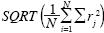, where r_j is the difference between the realizations mean and the true mean at point j, and N is the total number of points. For the covariance comparison the error is calculated as 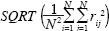where r_ij is the difference between the covariance (at positions i and j) calculated by the realizations and the true covariance.

For problem (2), when a three dimensional random hydraulic conductivity field is assumed, the behavior for different random seeds is analyzed. For each number of realizations we made five runs with different seeds. The deviations of each run from the true statistics were calculated.

 

Latin hypercube sampling

Latin hypercube sampling was developed to address the need for uncertainty assessment for a particular class of problems (Wyss and Jorgensen, 1998). Consider a variable Y that is a function of k statistically independent variables X¹, X²,... X^k and let F_j be the distribution of X^j, j=1,..., k. Latin hypercube sampling selects n different values from each of these k variables in the following manner (Owen, 1994):

where _j (1),..., _j(n) is a random permutation of 1,..., n in which n is the total number of realization, all n! outcomes are equally probable, U_ij is a U(0, 1) random variable, and the p permutations and np uniform variates are mutually independent. In other words, the LHS approach is characterized by a segmentation of the assumed probability distribution into a number of non–overlapping intervals, each having equal probability. From each interval a value is sampled at random.

The lattice sampling technique of Petterson (1954) is a special case of LHS. In lattice sampling, the F_j are discrete uniform distributions and n is a multiple of the number of atoms in each F_j . In this case the U_ij do no affect X_i^j , and they could all be taken to be .5 (Owen, 1994).

 

Sequential Gaussian simulation

Sequential Gaussian simulation (SGS) is a well–known stochastic simulation algorithm that is used to obtain Gaussian random fields (for a review of the theory see Deutsch and Journel, 1998). The algorithm we use herein was taken from GSLIB (Deutsch and Journel, 1998), a geostatistical software package developed at Stanford University.

 

Example 1

A random 1n K field, which is second–order stationary and isotropic, is assumed. Realizations are generated on a mesh with 27 x 27 square blocks, each block side is 100 m long, with two uniform layers of 150 m thickness each. The target correlation matrix is given by the autocovariance function for which we assume:

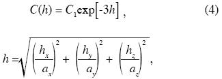
where C(h)is the covariance between two points separated by a distance h, h_x , h_y and h_z are the distances between the two points in the x, y and z direction, respectively; and a_x, a_y and a_z are the ranges in the x, y and z directions, respectively. Two ranges are considered: 672 and 2500 m (a_x = a_y = a_z), which are within the values of ranges reported for ln in K in the literature (Gelhar, 1993), and two and three dimensional analyses were done. For the 2D analysis we considered h_z = 0. The same 2D example is presented by Zhang and Pinder (2003).

 

Comparison of results for example 1

Figure 1 shows the comparison of the means of 1n K errors, of the realizations generated by LHS versus those of SGS in 2D. The lattice sampling technique of LHS is an unbiased, for this reason there are no errors for the means (Zhang and Pinder, 2003). Fig. 2 shows the comparison of the covariances of 1n K errors, of the realizations generated by LHS versus those of SGS in 2D. The curve LHS is smooth and convergent as the number of realizations increases and when the number of realizations are 800 or more, the error does not decrease significantly any more (the LHS RMSE order is 0.001). The SGS presents error higher than that of LHS, even when we have 1500 realizations, the SGS error is 0.026 if the range is equal to 672 m, and 0.034 if the range is equal to 2500.

Fig. 3 shows the comparison of the means of errors, for the realizations generated by LHS versus those of SGS in 3D. The means obtained by the LHS technique, always will present the same behavior; i.e., there are no deviations for the means. Figure 4 shows the comparison of the covariances of errors for the realizations generated by LHS versus those of SGS in 3D. The curve LHS is smooth and convergent as the number of realizations increases and when the number of realizations is 1500 or more the error does not decrease significantly any more (LHS RMSE order is 0.001). The SGS presents an error higher than LHS, even when we have 1500 realizations, the SGS error is 0.025 if the range is equal to 672 m, and 0.029 if the range is equal to 2500 m.

 

Example 2

A random 1n K field, which is second–order stationary an isotropic, is assumed. Realizations are generated on a mesh with 29 x 21 square blocks, each block side being 25 m long, with two uniform layers of 150 m thickness each. The target correlation matrix is given by the autocovariance spherical function for which we assume:

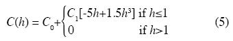
where C(h), C₀, h, a_x , a_y and a_z were defined earlier. For this example we considered C₀=0.3, σ²=C₀ + C₁=1.3 and two ranges, 672 and 2500 m. Also two and three dimensional analyses were done.

 

Comparison results for example 2

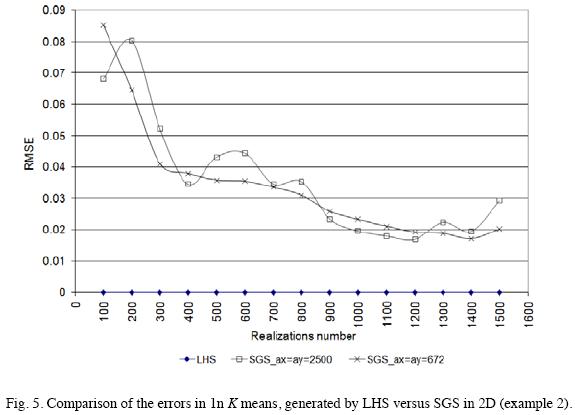
Fig. 5 shows the comparison of the means of 1n K errors, for the realizations generated by LHS versus those of SGS in 2D. Fig. 6 shows the comparison of the covariances of errors, generated by LHS versus SGS in 2D. The LHS curve is smooth and convergent as the number of realizations increases and when the number of realizations are 600 or more, the error does not decrease significantly any more (LHS RMSE order is 0.001). The SGS presents error higher than LHS, even when we have 1500 realizations, the SGS error is 0.043 if the range is equal to 672 m, and 0.044 if the range is equal to 2500 m.

Figures 7 and 8 show the comparison of the 1n K mean errors for ranges equals to 672 and 2500 m, respectively, generated by LHS versus SGS in 3D. As it was mentioned before, five different random seeds were used. With 1500 realizations the moments of SGS are clearly affected by the seed. Figs. 9 and 10 show the comparison of the errors in the 1n K covariances for ranges equals to 672 and 2500 m, respectively, generated by LHS versus SGS in 3D. Compared with the SGS method, the realization statistics of LHS are not affected significantly by the seed. We can consider that after 1300 realizations the LHS method is not affected by the seed. The LHS curves are smooth and convergent as the number of realizations increases and when the number of realizations is 1300 or more the error does not decrease significantly (The LHS error order is 0.001). The SGS presents errors higher than LHS, ranging between 0.037 and 0.064.

 

Conclusions

In the examples presented, the LHS method requires less realizations than the SGS method to converge.

For the example, in which an exponential autocova–riance function in 2D is considered, we can conclude that the LHS method converges after 800 realizations, because after 800 realizations the covariance matrix RMS error order is approximately equal to 0.001 and the changes on this error with extra realizations are very small.

For the example, in which an exponential autocova–riance function in 3D is considered, we conclude that LHS method converges after 1500 realizations, because after 1500 realizations the error order is approximately equal to 0.001 and the changes on this error with extra realizations are very small.

For the example in which a spherical autocovariance function in 2D is considered, the LHS method converges after 600 realizations, because after 600 realizations the error order is approximately equal to 0.001.

For the example in which an spherical autocovariance function in 3D is considered, we conclude that the LHS method converges after 1300 realizations, because after 1300 realizations the error order is approximately equal to 0.001.

We analyzed the effect of the seed for example 2 in 3D. Compared with the SGS method, the realization statistics of LHS are not affected much by the seed. We can consider that after 1300 realizations the effect of the seed for the LHS method is negligible because its magnitude is small and after this the error does not decrease significantly.

There are two important disadvantages of the LHS method in comparison with the SGS method. The first one is that if n₁ realizations are generated through the LHS method, the moments can be evaluated only after all the realizations are obtained. If the moments are not satisfactory, it is necessary to generate a complete new set of realizations, where n₂ > n₁. That is, it is not possible to accumulate the realizations in a sequential manner for the LHS method, while it is possible to accumulate them for the SGS method. The second disadvantage of the LHS method is that it has a large requirement of computer memory because it is necessary to store at least a NXNXN matrix, where N is the number of points to be generated and N_r is the number of realizations.

When working with stochastic flow and transport problems if the computer memory available is enough, it is recommended to use the LHS method because it can save a considerable amount of computational effort.

 

Acknowledgements

We want to thank Yingqi Zhang for providing us with the 2D LHS code which was modified to add the 3D option. RS greatly appreciate the support of CONACYT for a scholarship grant from February 2005 to February 2009.

 

Bibliography

Deutsch, C. V. and A. G. Journel, 1998. GSLIB Geostatistical Software Library and User's Guide, Oxford University Press, 369 p.         [ Links ]

Franssen, H. J. H., A. Alcolea, M. Riva, M. Bakr, N. V. D. Wiel, F. Stauffer and A. Guadagnini, 2009. A comparison of seven methods for the inverse modelling of groundwater flow. Application to the characterization of well catchments, Advances in Water Resources, doi: 10.1016/j.advwatres.2009.02.011.         [ Links ]

Gelhar, L. W., 1993. Stochastic Subsurface Hydrology, Prentice Hall, New Jersey.         [ Links ]

Harter, T., 1994. Unconditional and conditional simulation of flow and transport in heterogeneous, variably saturated porous media, Ph.D. thesis, University of Arizona.         [ Links ]

Herrera, G. and G. Pinder, 2005. Space–time optimization of groundwater quality sampling networks, Water Resources Research, 41, W12407. doi:10.1029/ 2004WR003626.         [ Links ]

Massmann, J. and R. A. Freeze, 1987. Groundwater contamination from waste management sities: the interaction between risk–based engineering design and regulatory policy. 1. Methodology, Water Resources Research, 23, 251–367.         [ Links ]

McLaughlin, D., L. B. Reid, S.–G. Li and J. Hyman, (1993), A sthochastic method for characterizing ground–water contamination, Groundwater, 31, 2.         [ Links ]

Orr, S., 1993. Stochastic approach to steady state flow in nonuniform geologic media, Ph.D. thesis, University of Arizona.         [ Links ]

Owen, A. B., 1994. Controlling correlations in latin hypercube samples, Journal of the American Statistical Association, 89.         [ Links ]

Sun, A. Y., A. Morris and S. Mohanty, 2009. Comparison of deterministic ensemble Kalman filters for assimilating hydrogeological data, Advances in Water Resources, doi:10.1016/j.advwatres.2008.11.006.         [ Links ]

Wong, H. S., and W. W–G. Yeh, 2002. Uncertainty analysis in contaminated aquifer management, Journal of Water Resources Planning and Management, 128,1, January 1, DOI: 10.1061/(ASCE)0733–9496(2002)128:1(33).         [ Links ]

Wyss, G. D. and K. H. Jorgensen, 1998. A User's Guide to LHS: Sandia's Latin Hypercube Sampling Software, Sandia National Laboratories, Albuquerque, N M 87185–0747.         [ Links ]

Zhang, D., 2002. Stochastic methods for flow in porous media, Academics Press, San Diego California, USA.         [ Links ]

Zhang, Y. and G. Pinder, 2003. Latin hypercube lattice sample selection strategy for correlated random hydraulic conductivity fields, Water Resources Research, 39, 8, 1226, doi:10.1029/2002WR001822.         [ Links ]