Articles

 

A simplified numerical approach for lateral spreading evaluation

 

J. M. Mayoral* and F. A. Flores and M. P. Romo

 

Instituto de Ingeniería, Universidad Nacional Autónoma de México, Del. Coyoacán, 04510 Mexico City, Mexico. ^*Corresponding author: JMayoralV@iingen.unam.mx.

 

Received: November 24, 2008
Accepted: June 3, 2009

 

Resumen

Los desarrollos ocurridos en las últimas décadas, tanto en los métodos numéricos de solución de problemas de ingeniería geo–sísmica, como licuación y sus efectos, así como en la tecnología computacional, ha permitido que el uso de técnicas rigurosas de modelado matemático sean más frecuentes en ingeniería aplicada. Sin embargo, para el caso particular de la estimación de desplazamientos laterales inducidos por sismos, (asociados a la licuación de áreas extensas de terreno), resulta complicado para llevar a cabo análisis detallados que involucren modelos bi y tridimensionales. Es común el recurrir a estimaciones estadísticas, o inclusive a predicciones obtenidas con sistemas neurodifusos. En este artículo, se introduce un enfoque simplificado para calcular los desplazamientos laterales inducidos por sismos cuando se presenta licuación. La respuesta dinámica de un perfil de suelo es simulada a través de elementos finitos unidimensionales acoplados a un esquema de generación de presiones de poro. La ecuación de movimiento se resuelve en el dominio del tiempo y con base en cada incremento de presión de poro. Los parámetros de resistencia y dinámicos del suelo se modifican, permitiendo la estimación de los desplazamientos del suelo que ocurren durante el evento dinámico. La formulación propuesta se aplica al análisis de varios casos de estudio en donde se realizaron mediciones de desplazamientos laterales.

Palabras clave: Licuación, presión de poro, carga cíclica, carga sísmica, desplazamientos laterales.

 

Abstract

Recent developments underwent in the last decades in both numerical methods as well as computer technology to be applied for solving geotechnical earthquake engineering problems, such as liquefaction and its related effects has allowed using rigorous modeling techniques more often in engineering practice, including finite differences and finite element. However, for the particular case of estimation of liquefaction–induced lateral displacements in large areas, it is cumbersome to perform detailed numerical analyses involving 2–D and 3–D models. Therefore, it is common to resort to statistical estimations or even to predictions obtained with neurofuzzy systems. In this paper, an alternative practice–oriented numerical approach is explored. The dynamic response of a soil profile is simulated by means of one dimensional finite elements coupled to a pore pressure generation scheme. The equation of motion is solved in the time domain and based on each pore pressure increment, both the shear strength and the dynamic soil parameters are modified, allowing estimations of soil displacements that occur during the dynamic event. The proposed formulation is applied to analyze several study cases for various earthquakes where actual lateral displacements measurements were available.

Key words: Liquefaction, pore pressure, cyclic loading, seismic loading, lateral displacements.

 

Introduction

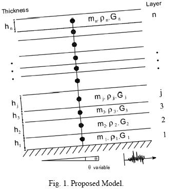
Seismic response evaluation of potentially liquefiable soil deposits is essential for a proper determination of the risk associated with ground movements, including cyclic mobility and lateral spreading, which can lead to significant damage in structural support elements of bridges, pipeline systems, harbors, as well as retaining structures during strong shaking. In general, the observed damage is directly proportional to the lateral pressures acting on the structural members, which in turn are proportional to the lateral displacements generated during an earthquake. For this reason, several researchers have proposed procedures to quantify lateral permanent displacements of the ground. These methods can be classified as (a) empirical methods, (b) knowledge–based field data procedures, and (c) mechanics–based methods. Several papers give a detailed account of the first two procedures (e.g., Barlett and Youd, 1992; Bazier and Ghorbani, 2005; Chiru–Danzer et al., 2001, and Wang and Rahman, 1999). The empirical methods are expressed in terms of statistical relationships. These relationships, however, have proven to be inadequate in several cases, mainly due to the limited and sometimes contradictory information with which they were developed (e.g., Cetin, 2004, and Garcia et al., 2007). Recently, methods based on neurofuzzy systems, which improve substantially the predictions of lateral permanent displacements, have been proposed to perform a better and more rational discrimination of the available data bases (e.g., Garcia et al., 2007). In the other end of the spectrum are the mechanics–based methods, which range in complexity from the simplest one proposed by Newmark (1965), to more complex dynamic procedures (e.g., Finn, 1990, and Cundall, 1995) passing through pseudostatic approaches (e.g., Bryne, 1981; Yasuda et al., 1990; and Yasuda et al. 1999). Although most mechanics–based methods have sound mathematical roots, their use is rather limited in practice, due mainly to the specialized knowledge needed to correctly define all soil parameters required to be input in the numerical solutions (basically finite differences and finite element methods). This paper is aimed at exploring the predictive potential of a simplified yet robust numerical approach, which allows the evaluation of the seismic performance of potentially liquefiable soil deposits. In this approach, a horizontally (or with a gentle inclination), stratified soil profile is simulated with one–dimensional finite elements (fig. 1). The equation of motion is solved in the time domain to account for nonlinearities in the stress–strain–pore pressure relationship, which is defined by a hyperbolic model coupled to a pore pressure generation scheme that assumes a linear dependency of the pore pressure with cyclic loading. Although it is well known that the hyperbolic model simplifies many features of the stress–strain behavior exhibited by soils, specially when the dynamic pore pressure is reaching the confining stress, and that the relationship between the increment in pore pressure during cyclic loading is in reality nonlinear, the main goal of this work was to provide a practice–oriented analytical tool that with very few parameters will lead to representative estimations of the lateral displacements induced by liquefaction, rather than to develop a multi–parametric sophisticated model able to represent the soil behavior observed in an element test in the laboratory but cumbersome to use for estimations of lateral spreading in practice. In this paper, the proposed approach was used to analyze several well documented case histories, including the lateral soil displacements occurred during the Kocaeli, Turkey, 1999 earthquake.

 

Proposed numerical scheme

The idealized numerical model depicted in fig. 1, was formulated to obtain the seismic response of the soil deposit. The wave propagation problem is solved in the time domain, considering SH–waves propagating vertically through a stratified soil deposit underlain by a half space, where the model base was assumed and the excitation is specified. The model uses a formulation based on finite elements with a linear variation of displacements in each element, to approximate the response of a shear beam. The finite element mesh is updated at every time step to approximately account for the large magnitude of displacements expected during liquefaction. The model can take into account an slightly slope inclination in the layered system, by decomposing the inertial component in a direction parallel and perpendicular to the sliding plane, so the effect of the constant shear force due to mild sloping base conditions are accounted for approximately. For sites where the slope inclination of the half space is important, the applicability of one dimensional analysis is limited, and a 2–D approach is required, such as that presented in Mayoral and Romo (2008).

The stress–strain relationship of the soil was represented with a hyperbolic model, however the shear strength of the soil and other dynamic parameters are modified according to the pore pressure build up during the earthquake, following the cyclic stress approach (e.g., Seed and Idriss, 1971). No pore pressure dissipation within the soil mass was allowed during the dynamic event. This condition, however, is deemed acceptable for the problem at hand, considering that liquefaction observed in those layers implied poor drainage conditions or none. The simulation allows obtaining the pore pressure evolution in the soil mass during and after the earthquake, determining the permanent deformations associated with cyclic loading. The dynamic analysis of the geological profile, in the finite element technique is utilized, requires solving the global equation of motion, commonly expressed in matrix form as:

Where [M], [C] and [K] are the global matrixes of mass, damping and stiffness, resulting from the assemblage of each individual element, and are the relative nodal accelerations, velocities, and displacements, with respect to the model base, and P(t) is the vector of dynamic load, which includes the downslope gravitational force. The nonlinear internal force is given by the term [K] {u}. During the dynamic event, the dissipation of hysteretic energy occurs through the nonlinear soil behavior. The small strain damping is given by the damping matrix, which is defined based on a Rayleigh type formulation. It is warranted to mention that this is only an approximation to the frequency independent damping, used in solutions formulated in the frequency domain, which does not have exact solution in the time domain. This is only used to estimate the damping at the beginning of the dynamic event. In subsequent times, the damping is characterized throughout the hysteretic soil response and the nonlinear force. The mass matrix was built using an average of the consistent and lumped mass matrices to better estimate the fundamental frequencies of the system, and to optimize the ability of the element to transmit high frequencies Romo et al. (1980). The time variation of the model is solved using the Newmark integration method.

 

Constitutive model selected for soils

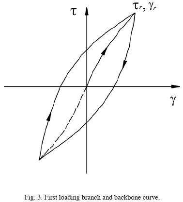
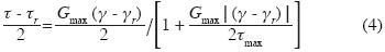
Although there is a number of sophisticated multi–parametric constitutive models available in the technical literature to represent the strain–stress–pore pressure relationship of liquefiable soils (e.g., Wang et al., 2006), to facilitate the application of the proposed numerical scheme in practice, a hyperbolic model (e.g., Konder and Zelasko, 1963) coupled with a pore pressure generation scheme was adopted. The model parameters can be fully defined from Standard Penetration Test, SPT, (for sandy materials) or Cone Penetration Test, CPT, (for clayey materials). Thus, the first loading branch is defined by the small strain shear stiffness G_max through the equation:

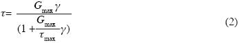
Where is the shear stress corresponding to an amplitude γ, and is the maximum shear stress that can be applied to the soil in the initial state without failure, as depicted in fig. 2.

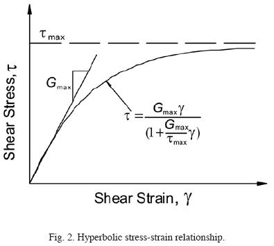
The unloading–reloading phase, shown in fig. 3, is given by the following expression:

Where γ_r and _r correspond to the unloading shear strain and stress respectively. Equation (3) can be written in explicit form as follows (e.g., Finn et al., 1975):

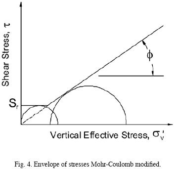
Clayey and unsaturated sandy soils were considered as purely hysteretic, without accounting for pore pressure generation, with a failure surface given by the Mohr–Coulomb criterion as:

Where is the vertical effective stress, and the parameters Φ and c are the friction angle and apparent soil cohesion of the soil. For saturated sands, the effect of the pore pressure generation was taken into account by reducing the shear strength of the soil as a function of the reduction in the vertical effective stress due to the increase in pore pressure due to cyclic loading and modifying the soil shear stiffness. Thus, the modified shear stiffness, G_mn, given by expression (6) will replace G_max in equation (4). The parameter G_mn is adjusted progressively for each change in vertical effective stress, in each time interval, Δt.

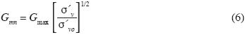
Here is the initial vertical effective stress, and is the vertical effective stress at the beginning of each cycle. These equations imply that the shear stiffness does not change importantly with variations in volumetric strain, ε_v, during cyclic loading (e.g., Finn et al., 1975). This assumption seems to better represent the behavior of potentially liquefiable soils, such as saturated finegrained sands, for the large shear strain levels associated with lateral spreading. As previously mentioned, no pore pressure dissipation within the soil mass was allowed during the dynamic event. After liquefaction, the shear strength of the soil is mostly provided by its residual strength, s_r. This was considered using a bilinear failure envelope defined by equation (5) but now replacing the parameter c with s_r. This envelope consists of an initial cohesion and friction value of zero, which extends until it intersects the Mohr–Coulomb envelope (Fig. 4). For steep sloping ground conditions, the residual strength is a key parameter assessing permanent displacement levels at the end of the earthquake. The residual strength can be estimated from Standard Penetration test, SPT, corrected for fines (N₁)_60–cs (e.g., Seed and Harder, 1990; and Idriss and Boulanger, 2007). The residual strength is the lower bound of shear strength, and will essentially define soil resistance when the pore pressure ratio, r_u, becomes 1.

 

Pore Pressure Generation Scheme

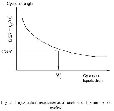
The cyclic stress approach was used to account for the pore pressure developed during cyclic loading. Thus, the liquefaction potential of a soil deposit is a function of the number and magnitude of the cyclic shear stresses acting on the soil during the dynamic event. These are measured in terms of the cyclic stress ratio (CSR), defined as the ratio between the cyclic shear stress _c divided by the vertical effective stress acting on the failure plane.

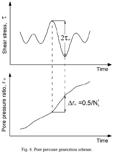
This relationship depends mostly on the seismic load, and is expressed in terms of the number of equivalent cycles. The number of equivalent cycles is defined by the duration intensity and frequency content of the earthquake, and the liquefaction resistance is expressed through a liquefaction resistance curve, which relates the number of cycles required to generate total liquefaction, with a uniform value of the cyclic stress ratio, as it is shown in fig. 5. The increment on pore water pressure Δu_g is expressed in terms of the so–called pore pressure ratio, . The computation of an increment of excess pore pressure is carried out based on the cyclic resistance strength curve, as illustrated in fig. 6. If N_Lⁱ uniform stress cycles are required to reach total liquefaction (i.e. when r_u becomes 1.0) for a given cyclic shear stress ratio CSRⁱ, then the increment in the pore pressure Δr_uⁱ for half a cycle will be 0.5/N_Lⁱ, and the corresponding increment in pore pressure Δu_gⁱ will be equal to . The increment in pore pressure reduces the vertical effective stress and, proportionally, the resistance to shear stress.

The curves of liquefaction resistance can be determined by laboratory testing (e.g., Seed and Idriss, 1971), or derived from CSR plots, which can be developed from the number of blows corrected by energy and fine contents, (N₁)_60–cs, obtained using Standard Penetration Tests, SPT, results.

 

Application of the proposed model

A performance evaluation of the proposed 1D model was done comparing its predictions with the response observed during three well documented case histories, the 1979 Imperial Valley, the 1987 Superstition Hills, and the 1999 Kocaeli earthquakes, in which small to large lateral displacements were observed (i.e. from 0.1 to 2.40 m).

 

The 1979 Imperial Valley and the 1987 superstitions hills earthquakes

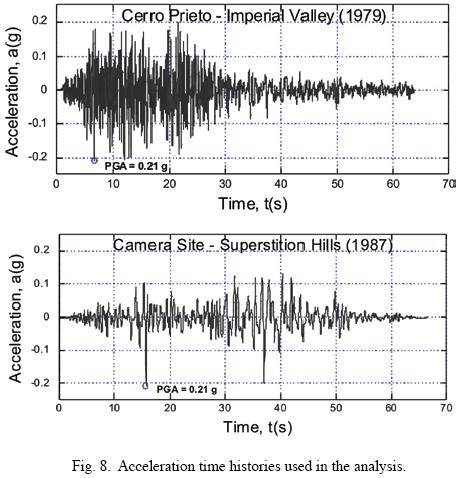
The 1987 Imperial Valley and 1979 Superstition Hills earthquakes occurred in California, United States. Both events had a magnitude M_w = 6.6, and caused liquefaction–induced lateral displacements at two sites, Wildlife and Herber Road, where several measurements were taken. Fig. 7 shows the location of these sites and the closest seismological stations placed on rock, which are identified as Camera Site and Cerro Prieto stations.

The first station is about 9 km away from Wildlife site. The second one is approximately 38 km away from Herber Road. Camara Site station and Cerro Prieto station registered the strong ground motions produced by the Imperial Valley and Superstition Hills earthquakes respectively. The corresponding acceleration time histories with the largest peak ground acceleration, PGA, recorded at the surface during both earthquakes are presented in fig. 8.

Subsoil conditions of studied sites and modeling

Several simplified 1–D models were generated for each of the cases compiled in Table 1. Cases C–1 through C–3 correspond to measures taken at Herber Road, and cases C–4 and C–5 to those taken at Wildlife, as indicated in fig. 7. According to the subsoil conditions found at each site as described by Bartlett and Youd (1992) these sites were comprised of a layer of saturated lose sand, with (N₁)_60–csranging from 2 to 10 and shear wave velocities lower than 200 m/s, resting on top of a more competent soil layer, that in all cases presented an slightly sloping upper boundary, defined by the angle θ, also included in Table 1. In each model, the soil strength was defined based on SPT –(N₁)₆₀ values corrected for fine contents. The acceleration time histories recorded on rock sites were deconvolved to the model base by means of one–dimensional wave propagation analysis using the program SHAKE–91 (Schnabel et al., 1972). In particular, the simplified stick model developed for case C–1, is presented in fig. 9, along with an idealized representation of the soil profile.

The hysteretic cycles and the corresponding accumulated permanent displacement computed at each depth are presented in fig. 10, as can be seen, most of the total permanent displacement occurred in the lower half portion of the soil deposit. Due to the highly nonlinear behavior exhibited by the liquefiable soil, the high frequencies are damped out, and in turn, the cyclic nature of the displacements becomes less notorious. Similar analyses were conducted for each case.

The computed displacement time histories at the surface, along with the permanent displacements, are summarized in fig. 11. This figure also includes the lateral measured displacements. A very good agreement between measured and computed response can be noticed for the cases analyzed.

 

The Turkey, 1999 Kocaeli Earthquake

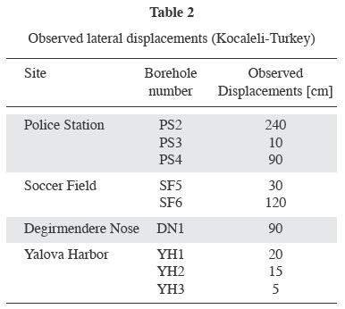
The model was used to estimate the displacement observed during the 1999 Kocaeli earthquake, which had a magnitude M_w=7.4. This event caused liquefaction–induced lateral displacements in the Izmit bay coast that were documented by several researches (e.g., Cetin et al., 2004), whom conducted post earthquake reconnaissance of the more affected sites, which included Police Station, Soccer Field, Degirmendere Nose and Yalova Harbor sites that are located in the south Izmit bay coast, as it is shown in fig. 12. A full description of the geologic setting and seismic environment prevailing at this region can be found in Cetin et al., 2004. The Izmit bay is located in an east–west trending active graben system which is dynamically affected by the interaction with the North Anatolian Fault Zone and the Marmara Graben System. The seismic event occurred along a 125 km segment of the North Anatolian fault (Fig. 12). Table 2 summarizes the lateral displacements measured at these zones.

 

Strong ground motions

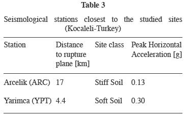
Figs. 13 and 14 present the acceleration time histories used in the analyses of these sites, which correspond to Yarimca and Arcelik stations. Table 3 compiles the information regarding these seismological stations, including the distance to the failure plane, soil type, and peak ground accelerations (PGA) observed during the Kocaeli, 1999, earthquake. Recordings from stations located in rock were not available during the analyses, which can be something very common in practice.

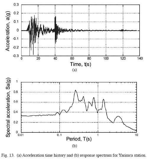
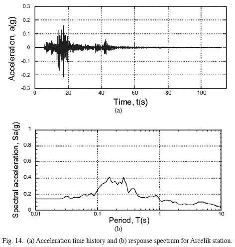
Thus, considering the proximity to the Police Station, Soccer Field and Degirmendere Nose sites, they were analyzed using the strong ground motion recorded at Yarimca station, and for the Yalova Harbor site, it was used the Arcelik station recording. It is warrant to mention that no significant soil nonlinearities occurred during this event, as can be deducted from the rather sharp peaks showing in the spectral shapes (figs. 13 and 14).

 

Subsoil conditions of studied sites and modeling

Again, as in the cases previously studied, several simplified models were generated based on the geotechnical information presented in Table 4, which was taken from Cetin (2004). In general, most of the sites studied were comprised by sand layers with SPT (N1)_60–cs values ranging from very low (i.e. 1 to 10) to relatively high values (i.e. larger than 50), interbedded with clay layers which thickness can vary approximately from 1 to 22 m. As an example, fig. 15 shows the idealized representation of the subsoil conditions found at Soccer Field, SF5, site and the model discretization.

The computed hysteretic cycles are presented in fig. 16, along with the accumulated permanent displacements at each depth. It can be noticed that most of the liquefaction occurs at the bottom of the sand layers which are located at the central portion of the soil profile, near the clay stratum. The upper sand stratum shows mostly a hysteretic response, without generating a large amount of excess pore pressure. The bottom clay layer presents a hysteretic response with a small contribution to the lateral permanent displacements. In all cases, the acceleration time histories were deconvolved again with a one dimensional wave propagation analysis to the model base using SHAKE–91, and the permanent displacements were computed at the surface with the proposed formulation.

Again, as can be seen in fig. 16, soil nonlinearities damped out the high frequencies of the input ground motions, and the permanent deformation component of the computed displacement time histories becomes more significant than the cyclic elastic component.

The lateral displacements obtained with the discrete model and those measured are compared graphically in fig. 17, including the lateral displacements obtained by Cetin, (2004) using Shamoto's (1998), Hamada's (1986), and Youd's (2002) methods. As can be seen in fig. 17, the results obtained with the proposed numerical scheme are closer to the observed displacements in the studied sites than those computed with the empirical models. It is clear that for larger displacements, the dispersion reduces, which can be attributed to a better characterization of the dynamic parameters in those sites where the most important failures occurred.

 

Conclusions

This paper introduces a practice–oriented numerical scheme to estimate earthquake–induced lateral spreading as an alternative to approaches based on statistical relationships. Regardless of the simplicity of the formulation, the model appears to have the capability of predicting fairly well the lateral ground movements observed in the case histories analyzed. Thus, although further comparisons with a larger number of cases will be desirable to asses the model performance fully, this simplified approach can still be used as guidance for estimating the order of magnitude of expected lateral displacements in both saturated and dry sands, as well as in clays. The better characterized are the subsoil conditions, including (N₁)₆₀, soil shear strength of clayey materials, and the input ground motions, the greater the accuracy the model predictionsare. Thus, the simplified numerical scheme represents an upgraded practice–oriented alternative to traditional methods based on statistical approaches for a similar level of application effort.

 

Bibliography

Bartlett, S. F. and T. L. Youd, 1992. Empirical analysis of horizontal ground displacement generated by liquefaction–induced lateral spreads, Tech. Rep. NCEER–92–0021, National Center for Earthquake Engineering Research, Buffalo, NY, August 17        [ Links ]

Bazier, M. H., and A. Ghorbani, 2005. Evaluation of lateral spreading using artificial neural networks, Soil Dynamics and Earthquake Engineering, Elsevier, 25, 1–9        [ Links ]

Bryne, P. M., 1981. A model for predicting liquefaction induced displacements due to seismic loading, Second International Conference on Recent Advances in Geotechnical Earthquake Engineering and Soil Dynamics, St Louis Missouri, paper No7.14, March, 1027–1035        [ Links ]

Cetin, K. O., I. Nihat and U. Berna, 2004. Seismically induced landslide at Degirmendre Nose, Izmit Bay during Kocaleli (Izmit)–Turkey earthquake. Soil Dynamics and Earthquake Engineering, 189–197        [ Links ]

Cetin, K. O., T. L. Youd, R. B. Seed, J. D. Bray, J. P. Stewart, H. T. Durgunoglu, W. Lettis and M. T. Yilmaz, 2004. Liquefaction–induced lateral spreading at Izmit Bay during the Kocaeli (Izmit)–Turkey Earthquake, Journal of Geotechnical and Geoenvironmental Engineering, ASCE, 130, 12, December        [ Links ]

Chiru–Danzer, M., C. H. Juang, P. A. Christipher and J. Suber, 2001. Estimation of liquefaction–induced horizontal displacements using artificial neural networks, Can. Geotech. J., 38, 1, 200–207        [ Links ]

Cundall, P., 1995. FLAC Manual version 3.3, ITASCA Consulting Group Inc, Trasher Square East, 708 South Third Street, Suite 310, Minneapolis, Minnesota 55415, USA        [ Links ]

Finn, W. D. L., K. W. Lee and G. R. Martin, 1975. An effective stress model for liquefaction. Journal of the Geotechnical Engineering Division, ASCE, 102, GT6, pp 169–198        [ Links ]

Finn, W. D. L., 1990. Analysis of post–liquefaction deformations in soil structures, H Bollón Seed Memorial Symposium Proceedings, May, BiTech Published, Ltd, Vancouver, BC, Canada, 291–311        [ Links ]

Garcia, S. R., M. P. Romo and E. Botero, 2007. A neurofuzzy system to analyze liquefaction–induced lateral spread, Soil Dynamics and Earthquake Engineering, doi:10.1016/j.soildyn.2007.06.014        [ Links ]

Hamada, M., S. Yasuda, R. Isoyama and K. Emoto, 1986. Study On Liquefaction Induced Permanent Ground Displacements, Report of the Association for the Development of Earthquake Prediction in Japan, Tokyo Japan        [ Links ]

Idriss, I. M. and R. W. Boulanger, 2007. SPT and CPT–based Relationships for the Residual Shear Strength of Liquefiable Soils, Earthquake Geotechnical Engineering, 4^th International Conference on Earthquake Geotechnical Engineering–Invited Lectures, edited by Kyriazis D. Pitilakis        [ Links ]

Konder, R. L. and J. S. Zelasko, 1963. A hyperbolic stress–strain formulation for sands, Proceeding, 2nd Panamerican Conference on Soil Mechanics and Foundations Engineering, pp 289–324        [ Links ]

Mayoral, J. M. and M. P. Romo, 2008. Geo–Seismic Environmental Aspects Affecting Tailings Dams Failures, American Journal of Environmental Sciences 4 (3): 198–208.        [ Links ]

Newmark, N., 1965. Effects of earthquakes on dams and embankments, Geotechnique, 15, 2, 139–160        [ Links ]

Romo, M. P., J. H. Chen, J. Lysmer and H. B. Seed, 1980. PLUSH: A computer program for probabilistic finite element analysis of seismic soil–structure interaction, University of California, Berkeley, USA. UCB/EERC–77/01        [ Links ]

Schnabel, B., J. Lysmer and H. B. Seed, 1972. SHAKE. A Computer Program for Earthquake Response Analysis of Horizontally Layered Sites, College of Engineering, University of Berkeley, CA. Rep., No. EERC 72–12.        [ Links ]

Seed, H. B. and I. M. Idriss, 1971. A simplified procedure for evaluating soil liquefaction potential, Journal of the Soil Mechanics and Foundations Division. ASCE,97, SM9, pp. 1244–1273        [ Links ]

Seed, H. B. and L. F. Harder, 1990. SPT–Based analysis of Cyclic Pore Pressure Generation and Undrained Residual Strength, in., Proceedings, H. Bolton Seed Memorial Symposium, J. M. Duncan (ed.), University of California, Berkeley, 2. 351–376        [ Links ]

Shamoto, Y., J. Zhang and K. Tokimatsu, 1998. New charts for predicting large residual post–liquefaction ground deformations, Soil Dynamics and Earthquake Engineering, 17, Elsevier, New York, pp. 427–438        [ Links ]

Yasuda, S., H. Nagase, H. Kiku and Y. Uchida, 1990. A simplified procedure for the analysis of permanent ground displacements, Conference Proceedings, Third Japan–US Workshop on Earthquake Resistant Design of Lifeline Facilities and Countermeasures for Soil Liquefaction, December 17–19, San Francisco, Ca, 225–236        [ Links ]

Yasuda, S., N. Yoshida, H. Kiku, K. Adachi and S. GOSE, 1999. A simplified method to evaluate liquefaction induced deformation, Proc Earthquake Geotechnical Engineering (ed P Seco e Pinto), Balkema, Rotterdam, 2, 555–566        [ Links ]

Youd, T. L., C. M. Hansen and S. F. Bartlett, 2002. Revised multilinear regression equations for prediction of lateral spread displacement, Journal of Geotechnical and Geoenvironmental Engineering, 128, 12, pp. 1007–1017        [ Links ]

Wang, J. and M. S. Rahman, 1999. A neural network model for liquefaction–induced horizontal ground displacement, Soil Dynamics and Earthquake Engineering, Elsevier, 18, 555–568        [ Links ]

Wang, Z. L., F. I. Makdisi and J. Egan, 2006. Practical applications of a nonlinear approach to analysis of earthquake–induced liquefaction and deformation of earth structures, Soil Dynamics and Earthquake Engineering, 26, 231–252        [ Links ]