


Servicios Personalizados
Revista
Articulo
 Inglés (pdf)
 Artículo en XML
 Referencias del artículo
 Enviar artículo por email
Indicadores
-
 Citado por SciELO
 -
 Accesos
Links relacionados
-
 Similares en
SciELO
Similares en
SciELO
Compartir

 Permalink
Geofísica internacional
versión On-line ISSN 2954-436Xversión impresa ISSN 0016-7169
Geofís. Intl vol.48 no.3 Ciudad de México jul./sep. 2009
Article
A suggested reverse geomagnetic polarity event from the Panga de Abajo magnetic anomalies in Mexicali Valley, Baja California, México
J. García–Abdeslem1* and M. López Guzmán2
1 Centro de Investigación Científica y de Educación Superior de Ensenada, División de Ciencias de la Tierra, Departamento de Geofísica Aplicada, km 107 Carretera Tijuana–Ensenada, 22860, Ensenada, Baja California, México *Corresponding author: jgarcia@cicese.mx
2 Goldcorp México, Proyecto Peñasquito, Av. Universidad 103, Fraccionamiento Lomas del Patrocinio, Zacatecas, 98068, Zacatecas, México.
Received: July 10, 2008
Accepted: March 17, 2009
Resumen
Las características de tres conjuntos de datos aeromagnéticos observados en Panga de Abajo, al NE de Baja California, México, su modelación inversa 3D y la información geológica disponible, sugieren el registro de eventos geomagnéticos de polaridad normal e inversa en cuerpos volcánicos de composición máfica que intrusionan la columna sedimentaria a unos 1500 m de profundidad.
Palabras clave: Anomalías magnéticas, modelación inversa 3D, magnetización normal e inversa, Baja California, México.
Abstract
From 3D inverse modeling and available geologic data, three aeromagnetic data sets observed at Panga de Abajo, NE Baja California, México, suggest geomagnetic events of normal and reverse polarity in volcanic intrusive bodies of mafic composition intruding the sedimentary column at about 1500 m–depth.
Key words: Magnetic anomalies, normal and reverse magnetization, 3D inverse modeling, Baja California, México.
Introduction
Extension and volcanism are closely–related geologic processes active during Neogene time in NW México. In Mexicali valley, NE Baja California (Fig. 1), extension has generated space to accommodate up to 6 km–thick sedimentary sequences as found in well logs in the region (Pacheco et al., 2006). Volcanic activity is inferred from high amplitude magnetic anomalies observed in aeromagnetic maps from Panga de Abajo (PDA). To the best of our knowledge the PDA magnetic field anomaly was first recognized by de la Fuente and Sumner (1974) in an aeromagnetic survey carried out at an altitude of about 600 m over the Colorado River delta, in a study of the structure, depth, and rock types of the basement in this region. The PDA magnetic field anomaly (Fig. 2a) reported by de la Fuente and Sumner (1974, Fig. 4, p.42) is shown in Fig. 2. It may be interpreted by 2D forward modeling, as caused by a mafic intrusive body (Fig. 2c) with a magnetic susceptibility of 0.0013 cgs (0.16 SI) located at a depth between 2 and 6 km below sea level. De la Fuente and Summer propose that magmatic activity from a spreading center generated the mafic intrusive body associated with the PDA magnetic field anomaly. This spreading center would be located between the Cerro Prieto and Wagner spreading centers proposed by Lomnitz et al. (1970).
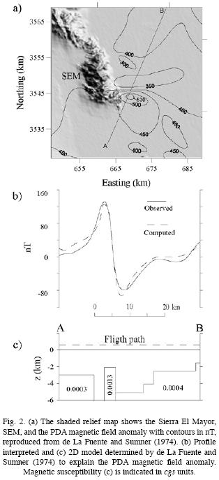

Fig. 1 shows an en echelon arrangement between the Cerro Prieto and Wagner spreading centers linked by the Cerro Prieto transform fault, as originally proposed by Lomnitz et al. (1970), and the PDA spreading center later proposed by de la Fuente and Sumner (1974), which preserves the right hand stepping of the en echelon arrangement of spreading centers and transform faults by adding an hypothetical right lateral transform fault, parallel to the trace of the Cerro Prieto fault that links the PDA and Wagner spreading centers.
In this work we refer to an interpretation by López–Guzmán (2003) of a second set of aeromagnetic data by the Instituto Mexicano del Petróleo (Ricardo Díaz Navarro, personal communication). This interpretation is based on 3D inverse modeling and suggests a possible reverse geomagnetic event in a mafic intrusive at the PDA site. A reverse geomagnetic event is suggested also from aeromagnetic data recently collected over the PDA site by the Servicio Geológico Mexicano (SGM). 3D inverse modeling of these new data, is based on a model that accommodates both normal and reverse magnetizations (García–Abdeslem, 2008). We take into account the interpretations by de la Fuente and Sumner (1974) and López–Guzmán (2003), plus available geologic data, to suggest that the PDA magnetic field anomalies are caused by volcanic bodies of probable andesitic or basaltic composition, that intrude the sedimentary column at about 1500 m–depth and which record normal and reverse magnetic polarities.
Surface geology and well data
The study area is located in the southern portion of Mexicali Valley (Fig. 3), within the physiographic province of the Gulf of California. It is part of the Colorado River delta. The valley is filled by semiconsolidated clastic sediments of deltaic and piedmont origin. The crystalline basement outcrops at Sierra El Mayor. It is a late Cretaceous granodiorite about 65 Ma old (Ortega–Rivera, 2003). It was exhumed in the Miocene between 15 and 10 Ma ago beneath a detachment fault (Axen et al., 2000). Overlaying the granodiorite, there are several outcrops of Paleozoic metamorphic rocks and Tertiary sedimentary rocks. Structurally, the Mexicali Valley is affected by the NW–SE striking Imperial and Cerro Prieto transform faults, which represent the boundary between the North American and Pacific tectonic plates (Fig. 1). The Cerro Prieto fault (Fig. 3) is located ~ 20 km east of PDA village.
There are no volcanic outcrops in Sierra El Mayor. Tertiary volcanic outcrops of basaltic composition are found in Sierra Las Pintas, about 20 km south of PDA village, and in Sierra las Tinajas, about 30 km to the southwest of the PDA site (Fig. 1). Quaternary lava flows and pyroclastic units of rhyodacitic composition outcrop at Cerro Prieto volcano (Quintanilla–Montoya and Suárez–Vidal, 1996), about 50 km north of PDA village (Fig. 1).
Several wells in the region show sedimentary sequences that were deposited initially during marine incursions from the Gulf of California and later by influx from the Colorado River (Pacheco et al., 2006). Two wells drilled by Petróleos Mexicanos (PEMEX, 1985) are shown in Fig. 3. Well W–3 bottoms out at 4500 m–depth in late Cretaceous–early Tertiary crystalline basement, classified as a granodiorite, with K–Ar age reported as 59 ± 5 Ma. Well W–2 ends at 3800 m–depth in a young volcanic intrusion, classified as an andesite, with K–Ar age reported as 1.4 ± 0.5 Ma. It cuts through several horizons of volcanic rocks between 1550 and 1880 m–depth.
Wells W–2 and W–3 are only ~ 30 km apart but their stratigraphic record (Fig. 4) shows remarkable differences. The lower stratigraphic sequence A in well W–3 is a marine shale of late Miocene age, as inferred from allochtonous planktonic foraminifera, which directly overlays the crystalline basement. The lower stratigraphic sequence A is absent in well W–2 which bottomed out in an andesitic lava flow. Overlaying the marine sequence A is the sequence B, shown in wells W–2 and W–3, which progressively grades up–hole into alternating mudstone–siltstone and sandstone beds. The deepest part of the sequence B in well W–3 is of late Miocene age, as inferred from autochthonous bentonic foraminifera. The main difference between wells W–2 and W–3 is in the sequence C, where sand intervals become progressively thicker and include conglomerate deposits. These deposits are thicker in well W–2, where gravel deposits are interstratified with lithic tuffs in the 1550–1880 m–depth interval, for which no ages are far available.
Rock magnetic properties
The depth of burial of the magnetized source bodies that cause the PDA magnetic anomalies rules out direct sampling to characterize its magnetic properties and its age. Measurements carried out on 16 samples of granodiorite outcropping in the region (García–Abdeslem et al., 2001) yield an average magnetic susceptibility of 14.3 x 10⁻⁴ (SI). Assuming an intensity of the local geomagnetic field of 48,000 nT, the induced magnetization in outcrops of granodioritic composition near the study area is of about 0.06 A/m.
A paleomagnetic study of the Cerro Prieto volcano by de Boer (1980) appears to be the only paleomagnetic study available nearby the study area. Cerro Prieto volcano (Fig. 1) is about 100 000 to 10 000 years old from paleomagnetic evidence which places it in the Pleistocene time, during the Brunhes chron of normal polarity.
Inverse modeling using juxtaposed prisms
López–Guzmán (2003) performed an interpretation of the PDAmagnetic field anomaly from a set of aeromagnetic data (Fig. 5a) collected ca. 1980, at an altitude of about 760 m above the sea level. Notice the low intensity of magnetic field anomalies observed over the Sierra el Mayor, as compared with magnetic field anomalies over the PDA site. As the crystalline basement outcropping at Sierra el Mayor and the basement found at the bottom of well W–3 is a granodiorite, with a low magnetic susceptibility, the source of the PDA magnetic anomaly may be a volcanic intrusion of mafic composition, as found at the bottom of well W–2 (Fig. 4), or as the intrusive of gabbroic composition that has been proposed as the heat source for the Cerro Prieto geothermal field (Goldstein et al., 1984; Quintanilla and Suárez–Vidal, 1994). Intrusive rocks of andesitic or basaltic composition have a magnetization of about 3 A/m (Carmichael, 1989).
López–Guzmán (2003) interpreted the PDA magnetic field anomaly by the Marquardt–Levenberg method of inversion (Marquardt, 1970; Levenberg, 1944). She used an expression for the magnetic field anomaly of a prism (Bhattacharyya, 1980). His subsurface model comprised 400 contiguous prismatic bodies with a regular cross section area of 2 by 2 km2. It was assumed that the prismatic bodies are uniformly magnetized with an intensity of 3 A/m along the local direction of the geomagnetic field. The field dips 50° to the north, and declination is 5° east of north. The problem is estimating depth to the top and bottom of the prisms.
The result of the inverse modeling performed by López Guzmán (2003) is shown in Fig. 5. The PDA magnetic anomaly is reasonably well fitted, with a maximum misfit of about 4 nT. The proposed source body is located at a depth of ~2.3 to ~3.95 km below sea level. Maximum thickness of the source body is about 1.65 km, but there is a zone of negative thickness (– 0.25 km) shown in Fig. 5 that was interpreted as due to localized reverse magnetization (López–Guzmán, 2003, López–Guzmán and García–Abdeslem, 2003). A negative thickness means that the top of a prism is deeper than its bottom; such an up side down prism causes a magnetic anomaly like that of a reversely magnetized prism. Notice that the negative thickness coincides with a relative minimun in the magnetic anomaly (Fig. 2a) as reported by de la Fuente and Sumner (1974, Fig. 4, p.42).
The new aeromagnetic data from SGM
The Servicio Geológico Mexicano (SGM) collected aeromagnetic data over the PDA site in drape mode at an altitude of 300 m above the terrain with N–S flight lines 1 km apart. These new data are shown in Fig. 6a. They tend to confirm the reverse magnetization event inferred by López–Guzmán (2003). In the following two sections we develop a preliminary interpretation of the PDA magnetic field anomalies from the aeromagnetic data collected by SGM.
Qualitative interpretation
Magnetic field anomalies describe the geometry of a magnetized body as it cooled below its Curie temperature. They depend on inclination (i) and declination (d) of the polarization vector in geomagnetic coordinates, as obtained from the local inclination (I) and declination (D) of the geomagnetic field. In appendix A we show some magnetic field anomalies caused by a single source body in a variety of conditions, including changes in the inclination and declination angles of the geomagnetic field and the polarization direction. Additional examples may be found in Bhattacharyya (1964).
Amplitude of the PDA magnetic field anomalies in Fig. 6a, correlation with surface geology, and magnetic susceptibility for the basement rocks exposed in Sierra el Mayor, suggest a mafic composition and a high magnetic susceptibility for the source bodies associated with the PDA magnetic field anomaly. The synthetic magnetic field anomalies with normal and reverse magnetization shown in appendix A suggest that a dipolar magnetic field anomaly like the one in the northern area (PDA–N) originated from a source body that cooled down to its Curie temperature and was magnetized at a time when the polarity of the geomagnetic field was reversed. Similarly, the dipolar magnetic field anomaly located in the south (PDA–S) suggests a source body that was magnetized at a time when the polarity of the Earth's magnetic field was normal.
Centroid depth using the AN–EUL method
Nabighian (1972) proposes that once a magnetic field anomaly has been selected for interpretation, and before attempting to model the data, semi–quantitative methods which require no prior assumptions might help infer the horizontal extension of the body and a preliminary estimate of its depth of burial. Some recent developments in semi–quantitative interpretation of magnetic anomaly infer depth to the top and the edges of the geologic target from the analytic signal (Li, 2006) or from 3D Euler deconvolution (Silva and Barbosa, 2003).
Combining analytic signal and the Euler method, Salem and Ravat (2003) have found a relationship for computing the centroid–depth z0 of the magnetized bodies

where  are the amplitudes of the nth–order derivative of the analytic signal (Debeglia and Corpel, 1997)

where the superscript z denotes the vertical derivative of the magnetic field anomaly T. In order to compute the centroid–depth from equation 1, the are evaluated at point (x0 , y0) where they reach a maximum value. This point is interpreted as the source's epi–centroid, which is located above the centroid of the source body.
The derivatives of the PDA magnetic field anomalies were computed from conventional Fourier transform techniques (Blakely, 1995). Comparing the PDA magnetic field anomalies with the (Fig. 6) clearly suggests that the magnetic field anomalies PDA–N and PDA–S are caused by two different source bodies. Taking into account the flight altitude (300 m above ground), the inferred centroid–depth below sea level is about 2.5 km in the case of PDA–S and about 2.2 km for PDA–N.
Inverse modeling of PDA magnetic field anomalies
The interpretation of the PDA magnetic field anomalies, as observed by the SGM was carried out using a method developed for 3D forward modeling (see Appendix A) and nonlinear inversion of the total–field magnetic anomaly caused by a uniformly magnetized layer with its top and bottom surfaces represented by a linear combination of 2D Gaussian functions (García–Abdeslem, 2008). The PDA magnetic field anomalies were analytically continued upward 1.5 km (Fig. 7a) and inversion was performed on the upward continued field following the Marquardt–Levenberg method (Marquardt, 1970; Levenberg, 1944).
In the following two sections we describe the results of the inverse modeling considering first that the source of magnetic field anomalies is a single layer normally magnetized in the direction of the local geomagnetic field, and secondly that the source of magnetic anomalies consists of two layers characterized by normal and reverse magnetizations, respectively.
Inversion assuming induced magnetization
We assume that the PDA magnetic anomalies are caused by a single layer, which is uniformly magnetized in the direction of the geomagnetic field, which locally has an intensity of about 48,000 nT, and it is characterized by an inclination angle of 50° down to the north and a declination angle of 5° east of the north. The magnetization intensity was set to 3 A/m, assuming a gabbroic or basaltic composition for the geologic target with an average magnetic susceptibility of 7.53 x 10⁻² (SI) (Carmichael, 1989).
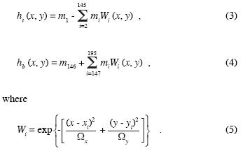
To carry out the inversion, 193 uniformly distributed Gaussian functions were used to simulate the top, ht , and bottom, hb , surfaces:
The spread of the Gaussian functions remain constant during the inversion: Ωx = Ωy = 16 for the upper surface, and Ωx= Ωy = 25 for the lower surface. The starting value for all of the model parameters, mi, was set to 0 km, and uncertainty of 0.25 nT was assumed in the magnetic data.
The results of the inversion are as shown in Fig. 7. The misfit between the observed and computed magnetic field anomalies varies between ± 5 nT. The depth to the top surface varies between 1.6 and 4.6 km below the sea level. The bottom surface is an elliptical feature that varies between 2.6 and 4.85 km–depth below the sea level. The maximum thickness is in the region of the PDA–S, where the layer is ~ 1.5 km thick, and it is minimum (~ 10 m) in the region of the PDA–N. As theoretically expected (Blakely, 1995, p 95, Fig. 5.6) the magnetized layer locally thins in the region where reverse magnetization is inferred.
Inversion assuming induced and remanent magnetization
To assess the possibility of remanent magnetization, the second model consists of two layers, uniformly magnetized in the presence of the earth's magnetic field. Taking into account the centroid–depth obtained using the AN–EUL method (Salem and Ravat, 2003), the bottom layer carries the magnetization in the direction of the present geomagnetic field, characterized by an inclination angle of 50° down to the north, and a declination angle of 5° east of the north. The top layer carries the magnetization in an opposite direction to the present geomagnetic field, with inclination angle i = –50°, and declination angle d = 185° and its lateral extension is limited to the vicinity of the PDA–N magnetic anomaly. The intensity of the induced and the remanent magnetizations were both set to 3 A/m.
In the two–layer model, the bottom layer is as described by equations 3 and 4, and the top layer is described by

The upper surface of the top layer was constructed using only nine Gaus sians with Ωx= Ωy = 1. The magnitude of induced and remanent magnetizations was set to J = 3 (A/m) in both layers. The starting value for all of the model parameters was set to 0 km, and an uncertainty of 0.25 nT was assumed in the magnetic data.
The results of the inversion are as shown in Fig. 8. Overall, the observed magnetic field anomaly was reasonably well fitted, and the misfit between the observed and computed magnetic anomalies varies between ± 3 nT. The depth to the top surface varies between 1.6 and 4.4 km below the sea level, and this surface shallows in regions coincident with both dipolar anomalies: its depth is ~ 1.5 km at the location of the PDA–S and ~1.4 km at the location of the PDA–N. The bottom surface is close to a circular feature that varies between 2.9 and 4.9 km depth below the sea level.
Fig. 9a shows the correspondence between the inferred top surface and the magnetic field anomaly map of the study area as observed by the SGM, and the source body is shown in a cross section (Fig. 9b) that includes the centroid–depths inferred using the AN–EUL method. We assume that the magnetic effect attributable to regional basement rocks of low magnetic susceptibility (de la Fuente and Sumner, 1974; García–Abdeslem et al., 2001) is accommodated by the inverse method varying the thickness of the normally magnetized bottom layer.
Discussion
The magnetized bodies that cause the PDA magnetic field anomalies are not accessible for direct sampling. Therefore, we discuss our interpretation using other independent information, which includes the regional tectonic framework (Suarez–Vidal et al., 2008, González–Escobar et al., 2009), the bio–stratigraphic record at wells W–2 and W–3 (Pacheco et al., 2006), and the magnetic polarity time scale of the phanerozoic (Ogg, 1995).
The Cerro Prieto and Wagner spreading centers are linked by the Cerro Prieto fault (Fig. 1), which is one of the main structures in the Mexicali Valley and it extends southward into the northern Gulf of California. The Cerro Prieto fault has been part of the Pacific–North America plate boundary for about the last 6 or 7 Ma (Oskin et al, 2001) and its present displacement, in right lateral sense, is of about 46 mm per year (González–García, 2004). As shown in Fig. 3, the PDA magnetic field anomalies and well W3 are located over the western side of the Cerro Prieto fault, on the Pacific plate, whereas well W–2 is over the eastern side of the Cerro Prieto fault, on the North American plate.
By assuming to first order, rigid deformation along the plate boundary represented by the Cerro Prieto transform fault, thus the distance between the Cerro Prieto and Wagner spreading centers has been invariant during the last 6 or 7 Ma. Therefore, we infer that volcanic activity recorded at well W–2 (Fig. 4) possibly was originated in a magmatic event nearby the Cerro Prieto spreading center. By similar arguments, the marine sedimentary sequence A in well W–3 (Fig. 4) probably was deposited near the Wagner spreading center, while sequences B and C were settled during their northwestward translation along the Cerro Prieto transform fault to reach its present position.
Assuming by its proximity (~ 20 km) that the stratigraphic record at the PDA site is equivalent to the stratigraphic record at well W–3 (Fig. 4), and considering both the depth of burial and the magnetization intensity of source bodies that explain the PDA magnetic field anomalies, inferred by the AN–EUL and inversion methods, we interpret that the PDA magnetic field anomalies are caused by volcanic intrusive bodies of mafic composition intruding the sedimentary column.
Taking into account the relative dating at well W–3 (Fig. 4) and the vertical distribution at depth of normal and reverse polarities of the PDA source bodies, inferred from both the AN–EUL and inversion methods, the age of magmatic activity at the PDA site must be younger than late Miocene, during whichever normal and reverse magnetic polarity changes occurring during the Gilbert, Gauss, or Matuyama chrons (Fig. 10).
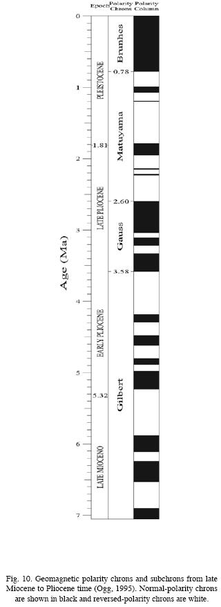
Outside of the Cerro Prieto and Wagner spreading centers, the volcanic intrusion in well W–2 (Fig. 4) is the only magmatic event recorded in the several deep exploratory–wells drilled in the region (Martín–Pacheco et al., 2006). If the age of the magmatic activity at the PDA site is equivalent to the age of the volcanic intrusive found at the bottom of well W–2, thus the normal and reverse magnetic polarities of the source bodies that cause the PDA–S and PDA–N magnetic field anomalies may be the result of geomagnetic field reversals occurring in late Pliocene–early Pleistocene time, during the chron Matuyama (Fig. 10).
Conclusions
Two out of three aeromagnetic data sets shown in figures 2a and 6 observed at different times and altitudes, and with different spatial resolution, and two inverse modeling interpretations shown in figures 3 and 8, performed on two different data sets, both suggest the presence of reverse and normally magnetized source bodies. The intensity of the magnetization (3 A/m) assumed for the source bodies in the inverse modeling and available geologic data, suggest that the PDA magnetic anomalies are caused by a mafic volcanic intrusive of possible andesitic or basaltic composition, intruding the sedimentary column at about 1500 m–depth. The depth of burial of the magnetized source bodies rule out direct sampling and the possibility of a hard bound on its age or magnetic polarization. Therefore, having non additional independent information the age of the PDA magmatic activity remains unknown.
Acknowledgements
We thank the generous help from Juan Contreras Pérez, José Manuel Romo Jones, and Gerry Connard, for reading and commenting the first draft of the present manuscript. Figures were made with the kind help of Victor M. Frías Camacho. We also acknowledge the positive and yet critical comments made by two anonymous reviewers that helped to improve the contents of this manuscript.
Bibliography
Axen, G. J., M. Grove, D. Stockli, O. M. Lovera, D. A. Rothstein, J. M. Fletcher, K. Farley and P. L. Abbott, 2000. Thermal evolution of Monte Blanco dome; Low–angle normal faulting during the Gulf of California rifting and late Eocene denudation of the eastern Peninsular Ranges. Tectonics, 19, 197–212. [ Links ]
Bhattacharyya, B. K., 1964. Magnetic anomalies due to prism–shaped bodies with arbitrary polarization. Geophysics, 29, 517–531. [ Links ]
Bhattacharyya, B. K., 1980. A generalized multibody model for inversion of magnetic anomalies. Geophysics, 45, 255–270. [ Links ]
Blakely R. J., 1995. Potential theory in gravity and magnetic applications: Cambridge University Press. New York. [ Links ]
Carmichael, R.S., 1989. Practical handbook of physical properties of rocks and minerals. CRC Press. [ Links ]
De Boer, J., 1980. Paleomagneti sm of the Quaternary Cerro Prieto, Crater Elegante, and Salton Buttes volcanic domes in the northern part of the Gulf of California rhombochasm. Proceedings of the second symposium of the Cerro Prieto geothermal field, Mexicali, B. C. Comisión Federal de Electricidad, pp 91–98. [ Links ]
De la Fuente, M. and J. S. Sumner, 1974. Estudio aeromagnético del Delta del Río Colorado, Baja California, México. Geofísica Internacional, 14, 35–48. [ Links ]
García Abdeslem, J., J. M. Espinosa–Cardeña, L. Munguia–Orozco, V. M. Wong–Ortega and J. Ramírez–Hernández, 2001. Crustal structure from 2–D gravity and magnetic data modeling, magnetic power spectrum inversion, and seismotectonics in the Laguna Salada basin, northern Baja California, México. Geofísica Internacional, 40, 67–85. [ Links ]
García–Abdeslem, J., 2008. 3D forward and inverse modeling of total–field magnetic anomalies caused by a uniformly magnetized layer defined by a linear combination of 2D Gaussian functions. Geophysics, 73, L11–L18. [ Links ]
Goldstein, N. E., M. J. Wilt and D. J. Corrigan, 1984. Analysis of the Nuevo León magnetic anomaly and its possible relation to the Cerro Prieto magmatic–hydrothermal system. Geothermics, 13, 3–11. [ Links ]
González–Escobar, M., C. Aguilar–Campos, F. Suárez–Vidal and Martín–Barajas, A., 2009. Geometry of the Wagner basin, upper Gulf of California based on seismic reflections. International Geology Review, 51, 133–144. [ Links ]
González García, J. J., 2004. Isla Guadalupe México (GUAX, SCIGN/PBO) a relative constraint for California borderland and northern Gulf of California motions. In AGU 2004 Fall Meeting. EOS, 85, p. F585. [ Links ]
INEGI (Instituto Nacional de Estadística Geografía e Informática), 2000. Datos geológicos vectoriales escala 1:250,000, Carta Mexicali (I1111). [ Links ]
Levenberg, K., 1944. A method for the solution of certain nonlinear problems in least squares. Quarterly of Applied Mathematics, 2, 164–168. [ Links ]
Li, X., 2006. Understanding 3D analytic signal amplitude. Geophysics, 71, L13–L16. [ Links ]
Lomnitz, C., F. Mooser, C. R. Allen, J. N Brune y W. Thatcher, 1970. Sismicidad y tectónica de la región norte del Golfo de California, México. Resultados preliminares, Geofísica Internacional, 10, 37–48. [ Links ]
López–Guzmán, M., 2003. Interpretación Mediante El método de la señal analítica y modelación inversa de la anomalía magnética "Panga de Abajo", Localizada al Sur de la Sierra El Mayor, Baja California, México. Tesis de Maestría en Ciencias, Centro de Investigación Científica y de Educación Superior de Ensenada. [ Links ]
López–Guzmán, M. y J. García–Abdeslem, 2003. Una estrategia para la interpretación 3–D de anomalías magnéticas. GEOS, 23, p.148 (resumen). [ Links ]
Marquardt, D. W., 1970. Generalized inverses, ridge regression, biased linear estimation and nonlinear estimation. Technometrics, 12, 591–612. [ Links ]
Nabighian, M. N., 1972. The analytic signal of two–dimensional magnetic bodies with polygonal cross–section: Its properties and use for automated anomaly interpretation. Geophysics, 37, 507–517. [ Links ]
Ogg, J, G., 1995. Magnetic polarity time scale of the Phanerozoic: in Online reference shelf 1, Global Earth Physics, a handbook of physical constants, (Tom Arens Ed.), American Geophysical Union. http://www.agu.org/reference/mainrefshelf.html [ Links ]
Ortega–Rivera, A., 2003. Geochronological constraints on the tectonic history of the Peninsular Ranges batholith of Alta and Baja California: Tectonic implications for western México. Geological Society of America, Special Paper 374, 297–735. [ Links ]
Oskin, M., J. Stock and A. Martín–Barajas, 2001. Rapid localization of Pacific–North America plate motion in the Gulf of California. Geology, 29, 459–463. [ Links ]
Pacheco, M., A. Martín–Barajas, W. Elders, J. M. Espinosa–Cardeña, J. Helenes and A. Segura, 2006. Stratigraphy and structure of the Altar basin NW Sonora: Implications for the history of the Colorado River delta and the Salton trough. Revista Mexicana de Ciencias Geológicas, 23, 1–22. [ Links ]
Petróleos Mexicanos (PEMEX), 1985, Proyecto de inversión San Felipe. Estudio de evaluación de cuencas. Informe RNCH–008, 57 pp. [ Links ]
Quintanilla, A. L. and F. Suárez–Vidal, 1994. Fuente de calor en el campo geotérmico de Cerro Prieto y su relación con la anomalía magnética de Nuevo León, México. Geofísica Internacional, 33, 575–584. [ Links ]
Quintanilla–Montoya, A. L. and F. Suárez–Vidal, 1996, Cerro Prieto y su correlación con los centros de dispersión del Golfo de California. Ciencias Marinas, 22, 91–110. [ Links ]
Salem, A. and D. Ravat, 2003. A combined analytic signal and Euler method (AN–EUL) for automatic interpretation of magnetic data. Geophysics, 68, 1952–1961. [ Links ]
Silva, J. B. C. and V. C. F. Barbosa, 2003. 3D Euler deconvolution: Theoretical basis for automatically selecting good solutions. Geophysics, 68, 1962–1968. [ Links ]
Suárez–Vidal, F., R. Mendoza–Borunda, L. M. Nafarrete–Zamarripa, J. Ramírez and E. Glowacka, 2008. Shape and Dimensions of the Cerro Prieto Pull–Apart Basin, Mexicali, Baja California, México, Based on the Regional Seismic Record and Surface Structures. International Geology Review, 50, 636–649. [ Links ]
Apendix A
The inclination (I) and declination (D) angles of the geomagnetic field, as well as the inclination (i) and declination (d) angles of the magnetization/polarization vector in uniformly magnetized source bodies and its geometry, strongly affect the characteristics of magnetic field anomalies. To show some of their characteristic, we use a method described in García–Abdeslem (2008) to compute several magnetic field anomalies caused by a uniformly magnetized body in the presence of the geomagnetic field.
The body is within a rectangular region bounded between the planes x = x1 and x2 along the northward x–axis, and between the planes y = y1 and y2 along the eastward y–axis. Along the z–axis, the body is bounded by ht (x, y) and hb(x, y), which define the top and bottom surfaces of the layer, respectively. These top and bottom surfaces are defined each by a linear combination of 2D Gaussian functions as
where m1,...,mM are constants, and
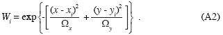
Each Gaussian function has unit amplitude at coordinates (xi , yi), and the spread of the function along the x– and y–axes is controlled by (Ωx , Ωy ).
The total field magnetic anomaly, T, at a point, r0, outside of the magnetic material, computed by the method described in García–Abdeslem (2008) was found by solving
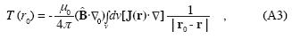
where r0(x0, y0, z0) is the point of observation, r(x, y, z) is the location of a volume element dv of the source body, Â is the unit vector parallel to the local direction of the geomagnetic field, J = Ji. + Jr is the total magnetization vector (sum of induced and remanent magnetizations) and µ0 is the magnetic permeability of free space.
The direction of the unit vector in the local direction of the geomagnetic field is defined by the director cosines L, M, N, where: L = cos I cos D, M = cos I sin D, and N = sin I. Similarly, the unit vector in the direction of the magnetization is defined by the director cosines l, m, n, where: l = cos i cos d, m = cos i sin d, and n = sin i.
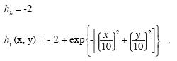
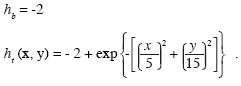
In the first example the base of the source body (hb) is flat at 2 km–depth, and its top surface (ht) is described by the 2D Gaussian function shown in Fig. A1:
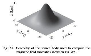
The magnetic anomalies shown in Fig. A2 were computed using a magnetization intensity of 1 A/m. In these examples the inclination of the geomagnetic field varies between 30 and 70 degrees and declination varies between –30 and 30 degrees. The several directions of the polarization vector used in these examples are listed in Table A1.It is worth to notice that all of the magnetic anomalies computed for this example show a dipolar signature. When the dip of inclination angles (I, i) is positive, magnetic anomalies are characterized by positive values on the south of the causative body, and by negative values on the north of the causative body, but the conversely happens when I is positive and i is negative. With an increase in the inclination angle (I), the negative anomaly, occurring on the north of the causative body reduces its amplitude, whereas the amplitude of positive anomaly on the south of the causative body increases.
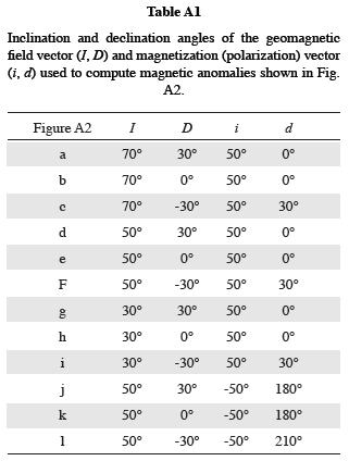
The direction along minimum and maximum is controlled by the declination angles, and several examples suggests that this direction is controlled by d at high inclination angles, I, whereas this direction is controlled by D at low inclination angles, I. The minimum and maximum values of the magnetic field anomalies are aligned in an N–S direction when D = –d.
Some other interesting cases occur when the aspect ratio (length / width) of the magnetized source body is grater than 1. We compute magnetic anomalies caused a source body with an aspect ratio of 3. The base of the source body (hb) is flat at 2 km–depth, and its top surface (ht) is described by a 2D Gaussian function:
The magnetic anomalies shown in Fig. A3 were computed using a magnetization intensity of 1 A/m. In these examples I = 50° and D is either 0° or 30° east of the north. The several directions of the magnetization vector used in these examples are listed in Table A2.

When magnetization vector is parallel to the direction of the geomagnetic field vector (I = i = 50°, D = d= 0°)the orientation of the long side of source body controls the location of the maxima and minima in magnetic field anomalies. Something similar happens if i = –I and d = D + 180°.
It is worth to mention that by the principle of superposition of potential fields (Blakely, 1985), magnetic anomalies observed in aeromagnetic maps seldom show the nice characteristics found in the computed magnetic field anomalies shown in this appendix. Magnetic field anomalies often consist of intense, long, and generally linear magnetic anomalies that originate from mafic extrusive or shallow intrusive igneous bodies, without dipolar signature.
Inclination and declination angles of the geomagnetic field vector (I, D) and magnetization (polarization) vector (i, d) used to compute magnetic anomalies shown in Fig. A2.
Inclination and declination angles of the geomagnetic field vector (I, D) and magnetization (polarization) vector (i, d) used to compute magnetic anomalies shown in Fig. A3, and orientation of the longest side (LSO) of the magnetized source body.

