Article

 

3D Simulations of the Quiet Sun Radio Emission at Millimeter and Submillimeter Wavelengths

 

V. De la Luz^1,*, A. Lara¹, E. Mendoza² and M. Shimojo³

 

¹ Instituto de Geofísica, Universidad Nacional Autónoma de México, Ciudad Universitaria Del. Coyoacán 04510 México City, México. E–mail: alara@geofisica.unam.mx* Corresponding author: vdelaluz@geofisica.unam.mx

² Instituto Nacional de Astrofísica Optica y Electrónica, Departamento de Astrofísica, Luis Enrique Erro # 1, Tonantzintla, 72880 Puebla, Mexico. E–mail: mend@inaoep.mx

³ Nobeyama Solar Radio Observatory/NAOJ/NINS, 462,2, Nobeyama, Minamimaki–mura, Minamisaku–gun, Nagano 384–1305, Japan. E–mail: shimojo@nro.nao.ac.jp

 

Received: September 30, 2007
Accepted: April 11, 2008

 

Resumen

Presentamos imágenes bidimensionales de simulaciones en 3D de la radioemisión solar en su régimen quieto a diferentes frecuencias, que van desde longitudes de onda centimétricas hasta submilimétricas (1.4, 3.9, 17, 34, 43, 110, 212 y 250 GHz). Construimos un modelo solar esférico 3D y resolvimos la ecuación clásica de transporte radiativo usando temperaturas y densidades electrónicas para el Sol Quieto. Comparamos nuestros resultados con observaciones del Nobeyama Radio Heliograph a 17 GHz. Las imágenes obtenidas a frecuencias de 3.9 GHz y 43 GHz serán de gran ayuda para calibrar las observaciones del nuevo telescopio milimétrico (RT5) que está siendo instalado en el Volcán "Sierra Negra", en el estado de Puebla, México, a una altitud de 4,600 m. Este proyecto es una colaboración entre el Instituto Nacional de Astrofísica Óptica y Electrónica (INAOE) y la Universidad Nacional Autónoma de México (UNAM).

Palabras clave: Radioemision solar, simulaciones de transferencia radiativa.

 

Abstract

We present 2D projections of 3D simulations of the quiet–sun radio–emission, at different frequencies on the centimeter–submillimeter wavelength range (specifically at 1.4, 3.9, 17, 34, 43, 110, 212 and 250 GHz). We have built a 3D, spherically symmetric, solar model and solved the classical equation of radiative transfer using quiet–sun temperature and electronic density models. We compare our results with Nobeyama Radio Heliograph observations at 17 GHz. The 3.9 and 43 GHz images will be useful to calibrate the observations of the new 5 meter millimeter telescope (RT5) which is going to be installed at "Sierra Negra" Volcano, in the state of Puebla, México, at an altitude of 4,600 m. over the sea level. This project is a collaboration between Instituto Nacional de Astrofísica Óptica y Electrónica (INAOE) and Universidad Nacional Autónoma de México (UNAM).

Key words: Solar radioemission, radiation transfer simulations.

 

Introduction

From the middle of the 20^th Century, models of quiet solar radio emission have been widely studied by Scheuer (1960), van de Hulst (1953), and Zheleznyakov (1965). As technology grew up, modern codes of these models were developed (Kuznetsova, 1978; Ahmad and Kundu, 1981). Nevertheless, these models predicted small scale structures, not observed at that time, as instance: the limb brightening at millimeter wavelengths. Some years later, the limb brightening was observed, however, models predicted higher brightness temperatures than the observed. Now a days, there is a considerable variety of both, theoretical (Landi and Chiuderi Drago, 2003) and empirical (Zirin et al., 1991) models attempting to reduce the discrepancy with the observations. Although, no one have solved definitively this problem. We present a 3D code of quiet Sun radio emission, called Pakal, (De la Luz et al., 2007), which helps to reduce this discrepancy. In particular, we present the 3D model of the quiet solar atmosphere and its resultant radio emission at different frequencies. This emission is projected into the plane of the sky, in order obtain 2D images which can be easily compared with observations. As an example, we present a detailed study of our model output at 17 GHz and compare our results with Nobeyama Radio Heliograph observations.

 

Method of Calculation

A code called Pakal was used in this work. Pakal is formed by four independent modules: I) the geometry model; II) the numeric radiative transfer model; III) the emission model and IV) numerical methods. Pakal is based on a 3D geometry where the origin is at the center of the solar sphere and the z axes is parallel to the Sun Earth line. So the amount of energy dI_v passing through an element of volume characterized by the distance ds is equal to the absorption I_vk_v plus the emission ε_ν inside the element, this is:

where k_v is the opacity function and ε_ν is the emission function. These functions depend on the emission and absorption processes inside the element ds. If we assume a plane parallel atmosphere

dx = cos (θ) ds = µds,

where dx is the geometric depth, θ is the angle between the observer and the vector perpendicular to the emission source layer. Using the Kirchoff law:

where S_v is called the source function, we get

where τ_v is the optical depth (dτ_v = –k_vdx). Taking into account only the component parallel to the line of sight (µ = 1), a constant source function, and integrating the optical depth using the trapezoidal rule we get the numerical solution of the specific intensity I_v , leaving the cell L_i+1as (De la Luz et al., 2007)

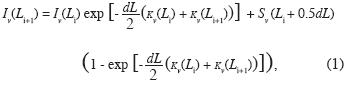
where L_i is a relative position in the specific geometry (the cell in the input layer), and dL is the integration step. We compute the emission due to free–free interactions between electrons and ions, based on the Dulk (1985) emission model for radio thermal emission:

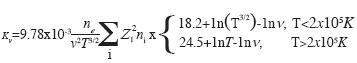
where n_e is the electronic density, ν is the frequency, T is the temperature, Z_i is the electric charge and n_i the density of the ion species "i". The radio thermal source function is

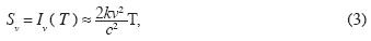
where k is the Boltzmann constant and c is the velocity of light.

 

Model of the chromosphere, transition zone and corona

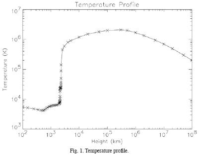
As inputs, Pakal needs three parameter profiles as a function of height: the temperature (Fig. 1), the Hydrogen density (Fig. 2), and the electronic density (Fig. 3). Another input is the percentage of ionization versus temperature. In this work we have used the temperature and Hydrogen density profiles for the Quiet Sun regimen, which were computed based on: the Vernazza et al. (1981) photospheric and high chromospheric models; the Gabriel (1976) coronal model; the chromospheric model (C) by Vernazza et al. (1981) and the Gabriel (1976) low coronal model published by Foukal (1990). The profiles for the transition region (TR) were interpolated between these models using lineal interpolation.

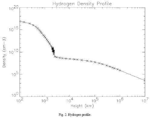
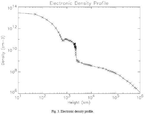
To compute the electronic density, we used the Vernazza et al. (1981) chromospheric model, but the transition region and low corona profiles were computed taking into account the electron contribution of Hydrogen and Helium in different ionization states:

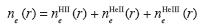
where n_e (r) is the electron density at height r above the photosphere, n_e^HII (r), n_e^HeII (r) and n_e^HeIII(r) are the electron density contributions of the different ions. To compute the electron density contribution of each ion, we have to know the possible states of ionization (in percentage) of each atom. We solve the classical Saha equation to get these values for a diatomic perfect gas with n(He) = 0.1n(H) and temperatures between 1,000K and 50,000K. Finally we have:

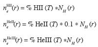
Where N_H(r) is the Hydrogen density at height r above the photosphere, %HII(T), %HeII(T), %HeIII(T) are the ionization percentages for HII, HeII and HeIII, respectively.

 

Results

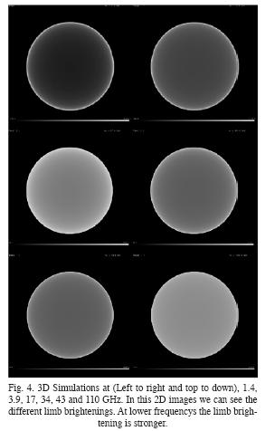
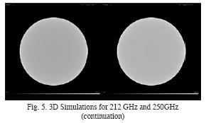
In this section we present the results of our model applied to the quiet–sun emission at 1.4, 3.9, 17, 34, 43, 110, 212 and 250 GHz. We have integrated the emission from –2R to 2R with a step integration of 0.5 km. The data files are available for download at http://cintli.igeofcu.unam.mx/vdelaluz/modelos. Fig. 4 shows the 2D projections of the simulated full disk emission at 1.4 (upper left), 3.9 (upper right), 17 (middle left), 34 (middle right), 43 (bottom left) and 110 GHz (bottom right). Similar results but for 212 (left) and 250 GHz (right) are a shown in Fig. 5.

 

Comparison with Nobeyama Observations at 17 GHz

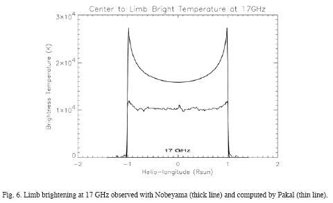
The Nobeyama Radioheliograph (NoRH) does not measure the absolute brightness temperature, it only measures variations of the brightness temperature. Therefore based on the findings of Zirin et al. (1991), the NoRH synthesis program assumes a brigthness temperature of 10,000 K at the disk center, on the other hand, our simulations can give information about the limb brightening computed at the solar equator (Fig. 6) and the height (or depth) of major emission in different ray path positions (Figs. 7 and 8). In Fig. 6 we show the comparison between Nobeyama observations at 17GHz and the prediction of the model using the same spatial resolution as the NoRH observations (~10 arcsec). The brightness temperature computed by the model is higher than the observed. The theoretical model expects an excess of 26,000 K at the zone of maximum emission, where as Nobeyama reports only an excess of 12,000 K in the same zone. At the center of the disk, the model predicts an excess of 16,000 k and Nobeyama reports 10,000 K, again less than the expected value. To investigate the origin of the differences between Nobeyama observations and Pakal model, we analyze in detail the emission process at different heights in two ray paths: one passing at the center of the disk and other passing trough the area of the highest intensity of the limb brightening. Fig. 7 shows the results of the ray path at the center of the disk, the zone of major contribution to the emission at 17GHz is marked with vertical dashed lines. The temperature profile (left upper panel) in this zone shows a growing stage, from 6,000 to 20,000 K. This increment in temperature produces an increment of ions and free electrons (Hydrogen is the mayor contributor in our model). In the right bottom panel, it is possible to see that the ion profile is different than the electron profile. This is one of the major differences between Pakal and previous works (Landi and Chiuderi Drago, 2003) where both profiles were assumed to be equal. This is very important due to the fact that the ion profile (lower right panel) traces the local emission profile (upper right panel). Fig. 8 shows the results of Pakal at the point of highest emission inside the limb brightening zone. In this case, the total emission profile (left central panel) is completely different than the same profile at the center of the disk. The emission does not begin on the solar surface, but behind the limb. In fact, there are two zones of high emission, the first one is at z = –0.05R but this emission is absorbed immediately as seen in the total emission profile (left central panel). A similar emission enhancement, which is not absorbed, takes place at z =0.05R , therefore, the observed emission comes from this thin layer. It is clear from the ions profile (see the "batman" profile in the right bottom panel of Fig. 8), that ions are responsible of this emission.

 

Summary and discussion

Pakal simulates solar radio–emission under the following assumptions: a layered plane–parallel atmosphere; local thermodynamic equilibrium; and in this (first) approximation, we have only taken into account the thermal emission due to electron–ion interactions, which is the main source of emission of radio waves (Dulk, 1985; Raulin and Pacini, 2005).

In this work we have used, as inputs, published profiles of temperature; electronic and Hydrogen densities; relative abundances; and opacities; we used also, well known source functions. Pakal model was applied to several frequencies in the mm and sub–mm wavelengths range to compute 2D projections of the 3D brightness distribution. These distributions show a limb brightening. However, at 17 GHz the model predicts higher brightness temperature in comparison to the observed one. It was found that the main contribution to this excess of brightness temperature comes from a layer of about 100 km thick, located at a 2100 km of height. We note that the spatial resolution of the input profiles (temperature and densities) at this height is of ~ 3 km (from 2104 to 2130 km over the photosphere). In this region the increment of temperature is considerable (from 9500 to 23000 K), whereas in the following 70 km, where the spatial resolution is ~ 30 km, the temperature increases only 1000 K. Therefore, the linear interpolation used in these regions is not a (numerical) source of over emission. It is important to note that this excess could be avoided by modifying the temperature and/or density profiles. However, it is not appropriate to arbitrarily modify them since they are supported by a fully developed theory.

It was found that the excess was larger for low frequencies and lower for high frequencies, and approaches to zero for frequencies higher than 43 GHz. This result is particularly interesting since previous models led to growing differences as the frequency increases. In particular, the chromospheric optical thickness at 17 GHz is very low above the 2210 km height. It is clear from Fig. 7 that the mayor contribution to the emissions comes from a layer below this height.

Among the possible reasons for the difference between our model predictions and the observed brightening, we mention the following:

1. The estimation of the opacity function may be wrong. Suprathermal particles can emit in ultra–violet (UV) but not in radio (Ralchenko et al., 2007) or the velocity distributions may not be a Maxwellian (Chiuderi and Chiuderi Drago, 2004).

2. The temperature profiles may be wrong due to a wrong calibration of the UV emission lines (Loukitcheva et al., 2004).

3. The electronic or Hydrogen density profiles are incorrect.

4. The magnetic pressure may be underestimated, i.e. there is not a hydrostatic equilibrium between the layers.

5. The abundances may be wrong. The abundances for the solar atmosphere may be overestimated (Yang and Bi, 2007; Avrett et al., 1976).

6. There is a lack of details in the computations. Some structures, as the spicules and coronal holes, have great influence on the radio emission (Wilhelm., 2006; Solanki., 2004; and Kuznetsova ,1978).

7. There may be absorption processes that have not been considered neither in previous models nor in ours (interplanetary plasma, opacity for other ions, etc.).

These reasons clearly show that there is a lot of work to do in order to improve the knowledge of the radio emission processes, particularly in the mm–range. In this way, one of the advantages of our model compared with previous works is the treatment of the ionic species densities. It was a common practice to approximate the ionic density to be equal than the electronic one. However, as it was seen in this work, the ionic density profile determines the behavior of the radio emission and is different of the electronic density profile. In order to determine the cause of the excess in brightness in our model, as future work, we are going to improve the solar model structure and include spicules. Up to now the spicules contribution to the emission has been considered as a filling factor, α. However, there is not a unique value for α. Different values have been adapted to fit the models with the observations. If we could characterize an inhomogeneous solar structure, it would be possible to estimate to what extent the filling factor is responsible for the excess in brightness.

 

Acknowledgments

Part of this work was supported by UNAM–PAPIIT grant IN118906 and CONACyT grant 49395. We thank to Dr. Rogelio Caballero from Instituto de Geofísica, of the Universidad Nacional Autónoma de México for giving us computing time in the Helios machine. We thank Nobeyama Solar Radio Observatory for the observational data at 17 GHz.

 

Bibliography

Ahmad, I. A., and M. R. Kundu, 1981. Microwave solar limb brightening, Solar Phys., 69, 273–287.        [ Links ]

Avrett, E. H., J. E. Vernazza and J. L. Linsky, 1976. Structure of the solar chromosphere. II – The underlying photosphere and temperature–minimum region, Astrophysical Journal Supplement Series, 30, 1–60.        [ Links ]

Chiuderi, C. and F. Chiuderi Drago, 2004. Effect of suprathermal particles on the quiet Sun radio emission, Astronomy and Astrophysics, 422, 331–336.        [ Links ]

De la Luz, V., A. Lara A and E. Mendoza, 2007. Modelación Tridimensional de la Atmósfera Solar en su Régimen Quieto para el Estudio de su Emisión en Radio, INAOE, Thesis.        [ Links ]

Dulk, G. A., 1985. Radio emission from the sun and stars, Annual review of astronomy and astrophysics, 23, 169–224.        [ Links ]

Foukal, P., 1990. Solar astrophysics, Wiley–Interscience, New York, 1990, 492 p.        [ Links ]

Gabriel, A. H., 1976. A magnetic model of the solar transition region, Royal Society of London Philosophical Transactions Series A, 281, 339–352.        [ Links ]

Griffits, D., 1999. Introduction to Electrodynamics, New Jersey, Addison–Wesley, 576 p.        [ Links ]

Hofman, J., 2001. Numerical Methods for Engineers and Scientis, Second Edition, Marcel Dekker Inc, 840 p.        [ Links ]

Kundu, M. R. and S. M. White, 1990. Millimeter and microwave activity of the sun, Basic plasma processes on the sun, Dordrecht, Netherlands, Kluwer Academic Publishers, 457–463.        [ Links ]

Kuznetsova, N. A., 1978. An inhomogeneous model of the chromosphere and lower corona for the interpretation of data on the radio emission of the quiet sun in the millimeter wavelength range, Soviet Astronomy, vol. 22, 345–349.        [ Links ]

Landi, E. and F. Chiuderi Drago, 2003. Solving the Discrepancy between the Extreme–Ultraviolet and Microwave Observations of the Quiet Sun, The Astrophysical Journal, 589, 1054–1061.        [ Links ]

Loukitcheva, M., S. K. Solanki, M. Carlsson and R. F. Stein, 2004. Millimeter observations and chromospheric dynamics, Astronomy and Astrophysics, 419, 747–756.        [ Links ]

Osterbrock, D., 1989. Astropysics of Gaseous Nebulae and Active Galactic Nuclei, USA, University Science Books, 408 p.        [ Links ]

Ralchenko, Y., U. Feldman and G. A. Doschek, 2007. Is There a High–Energy Particle Population in the Quiet Solar Corona?, The Astrophysical Journal, 659, 1682–1692.        [ Links ]

Raulin, J. P. and A. A. Pacini, 2005. Solar radio emissions. Advances in Space Research, 35, 739–754.        [ Links ]

Rohlfs, K., 1986. Tools of Radio Astronomy, Astronomy and Astrophysics Library, Germany, Springer–Verlag, 319 p.        [ Links ]

Scheuer, P. A. G., 1960. The absorption coefficient of a plasma at radio frequencies, Monthly Notices of the Royal Astronomical Society, 120, 231–241.        [ Links ]

Solanki, S. K., 2004. Structure of the solar chromospheres, Multi–Wavelength Investigations of Solar Activity, IAU Symposium, 223, 195–202.        [ Links ]

Van de Hulst, H. C., 1953. The Chromosphere and the Corona (The Sun), Gerard P. Kuiper. Chicago: The University of Chicago Press, 207 p.        [ Links ]

Vernazza, J. E., E. H. Avrett and R. Loeser, 1981. Structure of the solar chromosphere. III – Models of the EUV brightness components of the quiet–sun, Astrophysical Journal Supplement Series, 45, 635–725.        [ Links ]

Wilhelm, K., 2006. Solar coronal–hole plasma densities and temperatures, Astronomy and Astrophysics, 455, 697–708.        [ Links ]

Yang, W. M. and S. L. Bi, 2007. Solar Models with Revised Abundances and Opacities, The Astrophysical Journal, 658, L67–L70.        [ Links ]

Zheleznyakov, V. V., 1965. Model of the Lower Chromosphere Based on Radio Data, Soviet Astronomy, 8, 819–822.        [ Links ]

Zirin, H., B. M. Baumert and G. J. Hurford, 1991. The microwave brightness temperature spectrum of the quiet sun, Astrophysical Journal, 370, 779–783.        [ Links ]

Zombeck, 2006. Handbook of astronomy and astrophysics, 3 edition, United Kingdom, Cambridge University Press, p. 780.        [ Links ]