


Servicios Personalizados
Revista
Articulo
 Inglés (pdf)
 Artículo en XML
 Referencias del artículo
 Enviar artículo por email
Indicadores
-
 Citado por SciELO
 -
 Accesos
Links relacionados
-
 Similares en
SciELO
Similares en
SciELO
Compartir

 Permalink
Geofísica internacional
versión On-line ISSN 2954-436Xversión impresa ISSN 0016-7169
Geofís. Intl vol.47 no.3 Ciudad de México jul./sep. 2008
Article
Inter–decadal variability of Sporadic–E layer at Argentine Islands, Antarctica?
P. A. Flores1 and A. J. Foppiano2,*
1 Universidad del Bío–Bío, Casilla 5–C, Concepción, Chile. E–mail: pflores@ubiobio.cl
2 Universidad de Concepción, Casilla 160–C, Concepción, Chile. * Corresponding author: foppiano@udec.cl
Received: October 10, 2007
Accepted: January 21, 2008
Resumen
Se ha determinado las variaciones diurnas de la ocurrencia y de varias características de las capas esporádicas de la región E sobre Islas Argentinas (65.3°S; 64.3°W) para otoño, invierno, primavera y verano, tanto durante niveles de actividad solar baja como alta de los ciclos solares 21, 22 y 23. Se intenta identificar posibles variaciones interdecadales, aunque se usó equipos idénticos solo durante los ciclos 22 y 23. Parece haber diferencias reales entre ciclos, al menos para algunos tipos de Es en invierno.
Palabras clave: Esporádicas E, ionosfera, variaciones interdecadales, península antártica.
Abstract
The diurnal variations of Sporadic–E layer (Es) occurrence and of various Es characteristics over Argentine Islands (65.3°S; 64.3°W) have been determined for autumn, winter, spring and summer during both low and high solar activity level for solar cycles 21, 22 and 23. Although identical equipments were used only for cycles 22 and 23, an attempt is made to identify possible inter–decadal variations, which seem to have been documented for other locations. There seems to be true inter–cycle differences at least for some Es types during winter.
Key words: Sporadic–E, ionosphere, inter–decadal variability, Antarctic Peninsula.
Introduction
At mid–latitudes, Sporadic–E layer (Es) is the name given to charged metal ions that are swept into narrow layers (~1 to 5 km thick in vertical scale) by neutral wind shears usually in the height range 100–150 km (Whitehead, 1960, 1970, 1989; Mathews, 1998). Wind shears come from three wave sources, atmospheric gravity waves, tides and planetary waves. Es has strong diurnal and semi–diurnal variation of occurrence at mid–latitudes demonstrating the importance of atmospheric tides in the lower thermosphere (MacDougall, 1974, 1978). There is a growing body of evidence that there is a peak in the occurrence of gravity waves in the vicinity of the Antarctic Peninsula and to a lesser extent associated with the Andes (e.g. Espy et al., 2006; Preusse et al., 2006; Alexander and Teitelbaum, 2007; Baumgaertner and McDonald, 2007). The reason for this 'hot spot' is primarily due to orography, and the proximity of the Antarctic polar vortex. Es statistics can be a sensitive indicator of tides, planetary waves, gravity waves and their interactions. In this paper Es occurrence and Es characteristics are determined for given location in the Antarctic Peninsula sector (Argentine Islands) using ionosonde observations, manually scaled, and covering a three solar cycle interval. The main goal is to try to identify possible inter–decadal Es variability, as been suggested it exists for locations in the Australian sector (Baggaley, 1985), and which may lead to inter–decadal variability of the processes governing Es formation or destruction.
Data analysis
There are internationally–agreed standards for the analysis of vertical incidence ionosonde data. These are codified in Piggott and Rawer (1972 with further revisions in 1978). Here, the parameters determined at each hour are foEs, fbEs, h'Es and Es Type. foEs is the maximum frequency of an ordinary wave that can be reflected from an Es layer. The maximum frequency is related to the maximum ion concentration. fbEs is the lowest frequency at which the Es layer becomes semi–transparent. The difference between foEs and fbEs represents a measure of the spatial variation in the concentration of ionisation in the Es layer. h'Es is the virtual height of the Es layer. Es layer height determination is taken from the flat part of the trace. Because there is little underlying ionization the real height and the virtual height are normally very similar (probably within 5 km). For Es layers that show retardation effects, there will be greater uncertainty that is indicated by the qualifying letters. The minimum reflected frequency, fmin, was also determined. Es type is codified into four main classes at mid latitudes: f (flat) is the name given to all Es layers where there is no E layer present (i.e. at night), l (low) occurs below the height of the E layer, h (high) occurs above the height of the E layer, and c (cusp) lies between high and low types, i.e. within the E layer.
If foEs of a layer in the valley between the E and the F layer are less that foE, then the Es layer will not be detected by the ionosonde. Furthermore, as foE exhibits a diurnal variation, the 'visibility' of layers changes through the day. Both factors introduce an unknown bias into the analysis for the absolute occurrence of sporadic E layer. In spite of this limitation, the analysis proposed here is considered of some interest.
The international rules for ionogram interpretation allow up to three entries in the Es–type columns. The first entry is always the one from which the numerical Es parameters are determined. In the statistics presented in the paper, all three entries are used. However, it should be noted that having all three entries is not frequent.
Diurnal variations of Es occurrence and Es characteristics have been determined for solar cycles 21, 22 and 23 over Argentine Islands (65.2°S; 296°E geographic, –49.6; 8.84 corrected geomagnetic). Table 1 gives years used. The occurrences of the main four Es–types were determined simply counting the number of occasions a given type was present at a given hour. Diurnal variation are representative of autumn (February, March, April), winter (May, June, July), spring (August, September, October) and summer (November, December and January). The diurnal variations of foEs, fbEs, h'Es, and fmin for a given season are determined using monthly median values for all months grouped for that season. Simple average is computed using the three median values for a given hour.
Using identical equipment for all three solar cycles would have made the identification of possible inter–decadal variability much simpler. Unfortunately, during solar cycle 21 a different ionosonde was used (Union Radio Mark II – UR Mk II) than for cycles 22 and 23 (IPS 42). The UR Mk II ionosonde (Clarke and Shearman, 1953) was much more sensitive and it transmitted more power. Furthermore, the format of the ionograms was larger and thus it made it easier to scale. A comparison between data from co–sited earlier version of IPS 42 (designated 4A) and UR Mk II ionosondes has been reported by Rodger and Williams (1981). This means that gain sensitive para–meters (foEs and fbEs) would give slightly higher values during solar cycle 21 but other parameters (h'Es and Es type) will be unaffected, again provided no other effects exist. Also fmin would be lower during solar cycle 21.
As the solar activity differs from one solar cycle to another and possible Es inter–decadal variability may be associated to these solar activity differences, reference to solar activity indices are needed. Table 2 gives season mean values of daily flare index and of monthly mean sunspot numbers used. Season mean values of monthly mean geomagnetic Ap index are also given. Both flare indices and sunspot numbers indicate that solar activity for all three cycles is similar for winter and summer during low solar activity. For equinox at low solar activity and for high solar activity during all seasons solar activity is similar for cycles 21 and 22 but is significantly lower for solar cycle 23.
Results
Results for only the main four Es types, l, f, c and h, are determined since the percentage of occurrence for other types is very small when compared with those for the former. The fig. shows the diurnal variations of l and c Es–type percentage of occurrence for winter and summer at both low and high solar activity level. It should be noted that the scaling conventions determine the diurnal variation of some Es types, e.g. l has mainly a daytime occurrence while f has a night time occurrence. A summary of the main points determined from these figs. (and from figs. for f and h, and during equinox, not shown) is given in Table 3. Diurnal variations of fbEs and h'Es are also shown in the fig. Again, main features are summarized in Table 3 (including those from figs. for fmin and foEs, and during equinox, not shown).
The shapes of the diurnal variations of occurrence of l, f, c and h Es–types are almost the same during all three cycles for all seasons except for l type in summer at low and high solar activity. Otherwise, the inter–decadal variability is noticeably mostly on the amplitude of the diurnal variations. This is particularly so for l and c types although no consistent patterns arise. Some of the solar cycle 21 differences in the l type occurrence (larger) may be explained by the use of different equipment.
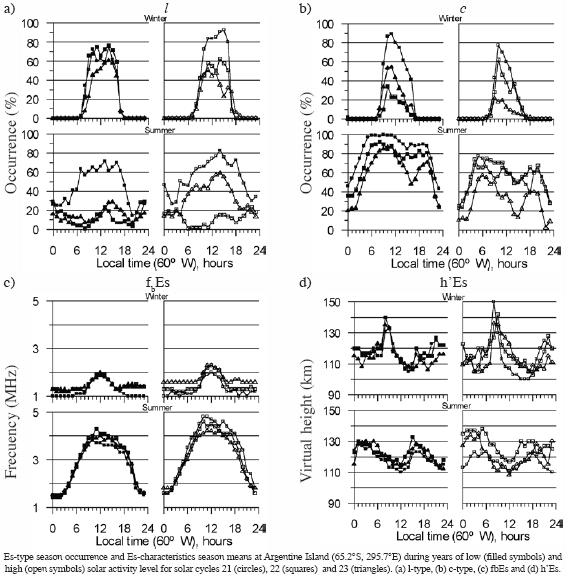
In the case of fmin, foEs, fbEs, and h'Es the shapes are similar in all cases. Again, it is the amplitude of the diurnal variations which shows some inter–decadal variability. For fmin some of the differences (lower at night of solar cycle 21) may also be associated to equipment and radio propagation differences. This allows lower values of foEs and fbEs to be read from ionograms. Very similar shape and diurnal amplitude for h'Es means that processes associated to Es formation or destruction do not change significantly from one solar cycle to another.
Although, as already mentioned, there is evidence of inter–decadal variations of Es parameters for locations in the Australian sector, the results of Baggaley (1985) cannot be directly compared with the results presented here.
Conclusions
There seems to be true inter–cycle differences for c Es–type occurrence although there is no consistent pattern for winter across solar activity level. The same may be true for l Es–type. Part of the differences in the amplitude of the diurnal variation may be associated to equipment differences.
It seems there is neither significant equipment nor inter–cycle differences for all Es parameter during low solar activity. The observed rather small inter–cycle differences during high solar activity do not seem to show a consistent pattern.
Acknowledgements
Data and preliminary data processing for Argentine Island were kindly offered by R. Stamper of WDC–C1, Appleton Rutherford Laboratory, Oxford, UK. Support for this study was provided by Fondo Nacional de Desarrollo Científico y Tecnológico under Proyecto No. 1010218.
Bibliography
Alexander, M. J. and H. Teitelbaum, 2007. Observation and analysis of a large amplitude mountain wave event over the Antarctic Peninsula, Journal of Geophysical Research, submitted. [ Links ]
Baggaley, W. J., 1985. Changes in the frequency distribution of foEs and fbEs over two solar cycles, Planetary and Space Science, 33, 457–459. [ Links ]
Baumgaertner, A. J. G. and A. J. MacDonald, 2007. A gravity wave climatology for Antarctica compiled from Challenging Minisatellite Payload/Global Positioning System (CHAMP/GPS) radio occultations, Journal of Geophysical Research, 112, D05103, doi:10.1029/2006JD007504. [ Links ]
Clarke, C. and E. D. R. Shearman, 1953. Automatic ionospheric height recorder, Wireless Engineer, 30, 211–212. [ Links ]
Espy, P. J., R. E. Hibbins, G. R. Swenson, J. Tang, M. J. Taylor, D. M. Riggin and D. C. Fritts, 2006. Regional variations of mesospheric gravity–wave momentum flux over Antarctica, Annales Geophysicae, 24, 81–88. [ Links ]
MacDougall, J. W., 1974. 110 km Neutral zonal wind patterns, Planetary and Space Science, 22, 545–558. [ Links ]
MacDougall, J. W., 1978. Seasonal variation of semidiur–nal winds in the dynamo region, Planetary and Space Science, 26, 705–714. [ Links ]
Mathews, J. D., 1998. Sporadic E: current views and recent progress, Journal of Atmospheric and Solar–Terrestrial Physics, 60, 413–435. [ Links ]
Piggott, W. R. and K. Rawer, 1972. U.R.S.I. Handbook of ionogram interpretation and reduccion, Second Edition, Report UAG–23, World Data Center A for Solar–Terrestrial Physics, NOAA, Boulder, Colorado. [ Links ]
Piggott, W. R. and K. Rawer, 1978. Revision of chapters 1–4 of the U. R. S. I. Handbook of ionogram interpretation and reduccion, Report UAG–23A, World Data Center A for Solar–Terrestrial Physics, NOAA, Boulder, Colorado. [ Links ]
Preusse, P., M. Ern, S. D. Eckermann, C. D. Warner, R. H. Picard, P. Knieling, M. Krebsbach, J. M. Russell III, M. G. Mlynczak, C. J. Mertens and M. Riese, 2006. Tropopause to mesopause gravity waves in August: Measurements and modeling, Journal of Atmospheric and Solar–Terrestrial Physics, 68, 1730–1751. [ Links ]
Rodger, A. S. and D. H. Williams, 1981. A comparative study of data from co–sited 4A and UR Mk II ionosondes, British Antarctic Survey, Internal Report number BAS/AS/ION/81/1(unpublished). [ Links ]
Whitehead, J. D., 1960. Formation of the sporadic E layer in the temperate zone, Nature, 188, 567. [ Links ]
Whitehead, J. D., 1970. Report on the production and prediction of sporadic E, Reviews of Geophysics and Space Physics, 8, 65–144. [ Links ]
Whitehead, J. D., 1989. Recent work on mid–latitude and equatorial sporadic – E, Journal of Atmospheric and Terrestrial Physics, 51, 401–424. [ Links ]

