Article

 

Measurements of upper mantle shear wave anisotropy from stations around the southern Gulf of California

 

S. A. C. van Benthem^1,2*, R. W. Valenzuela³, M. Obrebski^{4 , 5} and R. R. Castro⁴

 

¹ Department of Earth Sciences, Utrecht University, Budapestlaan 4, 3584 CD Utrecht, The Netherlands. ^*Corresponding author: benthem@geo.uu.nl

² Temporarily at Departamento de Sismología, Instituto de Geofísica, Universidad Nacional Autónoma de México, Mexico City, Mexico

³ Departamento de Sismología, Instituto de Geofísica, Universidad Nacional Autónoma de México, Mexico City, Mexico E–mail: raul@ollin.igeofcu.unam.mx

⁴ Departamento de Sismología, División Ciencias de la Tierra, Centro de Investigación Científica y de Educación Superior de Ensenada, Km. 107 Carretera Tijuana–Ensenada, 22860 Ensenada, Baja California, Mexico.

⁵ Dept. Sismologie, Institut de Physique du Globe, 4 Place Jussieu, 75252 Paris cedex 05, France

 

Received: November 29, 2007
Accepted: March 4, 2008.

 

Resumen

Se cuantificó la anisotropía sísmica del manto superior usando estaciones que rodean la parte sur del Golfo de California. El movimiento absoluto de la placa de América del Norte puede explicar las mediciones en la parte continental estudiada e implica que la litosfera arrastra al material de la astenosfera que se encuentra por debajo. Estas mediciones también son consistentes con la dirección de la extensión que ocurrió en la región de Cuencas y Sierras durante el Mioceno. Además las observaciones concuerdan con trabajos anteriores realizados en la región de Cuencas y Sierras, pero más al norte. El flujo astenosférico producido por la placa de Farallón subducida puede explicar la dirección anisotrópica rápida, orientada E–O, en el extremo sur de la península. Dicha explicación fue propuesta anteriormente para las estaciones de la mitad norte de la península. En la mitad sur de la península predominan valores de retraso pequeños y mediciones nulas. Estas mediciones difieren de las realizadas en el norte de la península. La existencia de fragmentos subducidos de las microplacas de Guadalupe y Magdalena podría explicar los pequeños valores de anisotropía observados. Una explicación alternativa podría ser el flujo ascendente de material caliente producido en la desaparecida dorsal de Magdalena ya que la placa subducida de Magdalena se había roto. La estación NE75, en la parte central de la península, parece registrar la transición entre los regímenes predominantes en el norte y el sur.

Palabras clave: Partición de ondas SKS, anisotropía del manto superior, flujo del manto, región mexicana de cuencas y Sierras, península de Baja California.

 

Abstract

Upper mantle seismic anisotropy was quantified at stations around the southern Gulf of California. Measurements on the mainland can be explained by the absolute motion of the North American plate, implying lithospheric drag of the asthenospheric material below. They are consistent with the direction of Basin and Range extension during Miocene time. These observations agree with previous work in the Basin and Range province farther north. The fast E–W anisotropic direction at the southern tip of the peninsula can be explained by asthenospheric flow produced by the subducted Farallón plate, as previously proposed for stations in the northern half of the peninsula. Small delay times and null measurements are dominant in the southern half of the peninsula in contrast with observations in the northern peninsula. The observation of low anisotropy may be caused by the subducted fragments of the Guadalupe and Magdalena microplates. Alternatively, it could be explained by upwelling of hot material from the former Magdalena ridge through the broken Magdalena slab. Station NE75, in the middle of the peninsula, appears to record the transition from the northern to the southern domain.

Key words: SKS splitting, upper mantle anisotropy, mantle flow, Mexican basin and range, Baja California peninsula.

 

Introduction

The minerals that make up Earth's mantle are anisotropic on a microscopic scale because of crystal structure. Many belong to the orthorhombic system and others to the monoclinic system. If the structure of a large number of crystals becomes preferentially oriented, anisotropy will be observed on a macroscopic scale. Alignment of the crystal axes gives rise to seismic wave velocity anisotropy (Hess, 1964; Nicolas and Christensen, 1987), in analogy with the birefringence of electromagnetic waves propagating at different speeds within a calcite crystal.

Three different mechanisms have been proposed to explain the orientation of upper mantle minerals (Silver and Chan, 1991). (1) Deformation produced by the motion of tectonic plates, which is very common in ocean regions (Raitt et al., 1969; Forsyth, 1975; Montagner and Tanimoto, 1990), (2) crustal stresses, and (3) past and present internal deformation of the subcontinental upper mantle, as produced by tectonic events (Silver and Chan, 1988, 1991; Silver and Kaneshima, 1993; Wysession et al., 1996; Vauchez and Barruol, 1996; Barruol et al., 1997). This mechanism best explains anisotropy observations in continental regions (Silver and Chan, 1988, 1991; Silver and Kaneshima, 1993). This means that orogenic and rifting events which control the orientation of continental geologic structures can also affect upper mantle structure (Silver and Chan, 1991). For mountain ranges and volcanic chains, and for areas of continental collision, the axis of fast seismic velocity becomes parallel to the tectonic feature (Silver, 1996). For extensional regimes, such as rifts and midocean ridges, the fast axis becomes parallel to the extension direction and perpendicular to the axis of the tectonic structure (Silver, 1996). For strike–slip motion the fast axis becomes parallel to the structure, i. e. the trace of the fault (Silver, 1996).

An important observation is "fossil" anisotropy. For regions which are no longer tectonically active, upper mantle anisotropy can be preserved for hundreds of millions of years (Silver, 1996). On the other hand, where no tectonic deformation has taken place, the axis of fast seismic velocity is often parallel to the direction of absolute plate motion (Savage, 1999). Additionally, anisotropy measurements in subduction zones have been used to study the effect of subducted slabs on mantle flow. Fischer et al., (2000) modeled mantle flow in the Tonga subduction zone back arc. Hall et al., (2000) focused on the Tonga, southern Kuril and eastern Aleutians subduction zones. Peyton et al., (2001) assumed that the fast direction of anisotropy tends to align parallel to the flow direction. They determined that mantle flow is trench–parallel at stations above the subducting slab in southern Kamchatka. Near the tattered slab edge, however, asthenosphere flows from beneath the subducting slab to beneath the overriding plate. Under the same assumption, for the Chile–Argentina subduction zone, Anderson et al. (2004) found mantle flow normal to the trench in areas where the subduction angle is shallow, whereas flow becomes parallel where the subduction angle steepens.

Anisotropy has been studied using the core phases SKS, SKKS, and PKS, as the path of these waves runs partly through the Earth's liquid, outer core (Silver and Chan, 1988, 1991; Silver and Kaneshima, 1993; Silver, 1996; Wysession etal., 1996; Vauchez and Barruol, 1996; Barruol et al., 1997; Savage, 1999; Fouch et al., 2000). Some experiments have shown significant differences in anisotropy when moving from a particular tectonic region to an adjoining one, e. g. near the Canada–United States border (Silver and Kaneshima, 1993), in Tibet (McNamara et al., 1994), and in the northeastern United States (Wysession et al., 1996; Fouch et al., 2000). In Mexico, Van Benthem (2005) quantified the anisotropy parameters under the broadband stations operated by the Servicio Sismológico Nacional (SSN; National Seismology Bureau) and under the southern half of the NARS–Baja California array. He showed that anisotropy under some stations in central and southern Mexico, a region with a complex tectonic environment, can be explained by the absolute motion of the North American plate. Obrebski et al., (2006) and Obrebski (2007) worked in the northern Baja California peninsula and in the northwestern portion of the Mexican Basin and Range. For the Basin and Range Province (east of the Gulf of California) their measurements agree with the absolute motion of the North American plate and with the direction of extension during the Miocene. In the northern Baja California peninsula, the fast direction of anisotropy is approximately E–W. This pattern may result from past asthenospheric flow induced by the sinking fragments of the Farallon plate, as proposed earlier by Özalaybey and Savage (1995) to explain a similar and probably related E–W pattern observed along the southwestern US borderland. This study presents some shear wave splitting measurements using stations installed around the southern Gulf of California, to the south of the area surveyed by Obrebski et al., (2006) and Obrebski (2007).

 

Data And Procedure

Most anisotropy measurements in this study used the SKS phase (downgoing S transmitted as P through the outer core and converted to S again for the upswing path) at epicentral distances greater than 90°. For distances less than 82° the first strong arrival on the radial component is the direct SV wave (Lay and Young, 1991) and is followed by SKS. At a distance of 82°, however, the SKS phase overtakes the direct SV (Lay and Young, 1991). Beyond 90°, SV and SKS have become clearly separated. Additionally, other core–mantle boundary (CMB) phases such as sSKS, SKKS and PKS were used as available. Clear SKS readings at these distances required a minimum magnitude of 6.0. The records were provided by Mexico's Servicio Sismológico Nacional (SSN) broadband network (Singh et al., 1997; Valdés González et al., 2005) and by the NARS–Baja California array (Trampert et al., 2003; Clayton et al., 2004). The SSN database was searched in the period from June 1998 to December 2003. A total of 35 earthquakes were obtained from La Paz (LPIG), and 239 events from Mazatlán (MAIG) within the distance and magnitude criteria. Stations in the NARS–Baja California array south of parallel 29°N provided 64 earthquakes for this study during the period from April 2002 to October 2004. Local problems with the equipment precluded the recording of some events at all stations. In all cases, the data were sampled 20 times per second using Streckeisen STS–2 broadband, three–component velocity sensors. Fig. 1 shows the study area and the location of the stations used.

The use of SKS phases to quantify anisotropy has several advantages. Because of P to S conversion at the CMB, the SKS phase is radially polarized. Therefore, SKS energy on the transverse component is a possible sign of mantle anisotropy in the upswing path on the receiver side. Care must be taken to ensure that the energy recorded on the transverse component is not due to scattering (Savage, 1999). SKS is a teleseismic phase that can be used to quantify anisotropy in regions with low or no seismic activity. It has a good lateral resolution, about 50–100 km, because its incidence is nearly vertical (Silver and Chan, 1991; Silver, 1996). While the vertical resolution is poor, most studies have found little anisotropy at depths greater than 400–600 km below the Earth's surface (Silver, 1996; Savage, 1999). It seems likely that anisotropy resides in the shallow part of the upper mantle, down to ~200 km depth, but the use of other kinds of data, such as surface waves, is necessary to confirm this for specific regions (Silver, 1996; Savage, 1999). Anisotropy has also been observed in the crust using the birefringence of local S waves (Crampin and Lovell, 1991) or receiver functions (Peng and Humphreys, 1997; Savage et al., 2007; Obrebski and Castro; 2008). The measured delay times in the crust typically range between 0.1 and 0.3 s, with an average of 0.2 s (Silver and Chan, 1991; Silver, 1996; Savage, 1999). For comparison, delays from SKS splitting go from barely detectable (0.3–0.5 s) to 2.4 s, and average to a little above 1.0 s (Silver, 1996). Contributions to delay times from the transition zone and the lower mantle are less than 0.2 s (Silver, 1996).

The procedure used in this paper to measure anisotropy was explained by Silver and Chan (1991) and is presented here only briefly. Upper mantle anisotropy beneath the seismometer leads to the observation of two SKS phases and is known as shear wave splitting. The early arrival is recorded in the fast horizontal component while the late arrival is recorded in the slow component. The difference between arrival times is known as the delay time, δt. The fast and slow components are orthogonal. In general, these are not identical to the radial and transverse components, which are also orthogonal. A second parameter is necessary to quantify anisotropy. Φ is the angle between the fast polarization direction and a reference direction, usually geographic north. In order to obtain the two parameters describing anisotropy, a time segment containing the SKS arrival, or another P to S CMB conversion, is selected from the north–south and east–west horizontal components. The two components are rotated by one degree at a time, with Φ ranging between –90 and 90°. For each value of Φ, the components are time shifted relative to each other using increments of 0.05 s, with δt ranging from 0 to 8 s. For each combination of Φ and δt, the eigenvalues λ₁ and λ₂of the covariance matrix between the two orthogonal components are evaluated. In the presence of anisotropy, λ₁ and λ₂ will be different from zero. Additionally, in the presence of noise, the desired solution will be given by the matrix which is most nearly singular. This is found by choosing the minimum eigenvalue, λ₂^min, from all combinations of (Φ, δt) within the space of possible solutions. In other words, the values of (Φ δt) associated to λ₂^min characterize the anisotropy because the highest cross–correlation within the given space occurs for the fast and slow waveforms. For interpreting the results, several special cases should be considered. (1) δt = 0 s indicates the absence of anisotropy. (2) Φ = Φ_b means that the fast axis, Φ, is oriented with the back azimuth, Φ_b . (3) Φ = Φ_b + 90° means that the fast axis is perpendicular to the back azimuth. Any of these three situations produces a null measurement and splitting of the shear wave cannot be detected.

Fig. 2 shows the SKS arrival on the radial and transverse components at SSN station MAIG for the earthquake of April 8, 1999 in the Japan Subduction Zone. The hypocenter was located at 560 km depth and the epicentral distance was 95.37°. Table 1 lists the events used in this study to quantify upper mantle anisotropy. Each SKS waveform was chosen by visual inspection and a first order, bandpass Butterworth filter was applied. In every case an attempt was made to retain the broadest bandpass possible, but the actual corner frequencies were determined based on the frequency of the noise affecting each record. The low frequency corner was chosen in the range from 0.01 to 0.04 Hz (periods between 100 and 25 s) while the high frequency corner varied between 1.0 and 1.5 Hz (from 1 to 0.67 s). These corner frequencies are appropriate for the phases used and the expected delay times (Wolfe and Silver, 1998). A time segment including only the selected phase was cut from the seismogram. In Fig. 2 the time series is 32 s long and is typical of the record lengths used throughout this work. Figure 3 shows the combination of (Φ, δt) producing the minimum eigenvalue, λ₂^min. The black dot means that the delay time, δt, is 0.95 s and the fast axis, Φ, is 74° east of north. The first contour around the dot bounds the 95% confidence interval for the measurement. All the other contours are multiples of the first one and are located at higher "elevations" or mountains. The black dot is located at the bottom of a valley. The 95% confidence contour was calculated using Equation (16) in Silver and Chan (1991) and taking one degree of freedom for each second of the record containing the SKS arrival (Silver and Chan, 1991; K. M. Fischer, Brown University, personal communication, 1998). The uncertainties are read directly from the contour plots. In this case, the measurement with its ±1σ uncertainty is (Φ, δt) = (74±20°, 0.95±0.45 s). In the event that the 95% confidence region is not approximately symmetric, the largest of the two possible 1σ values is used, e. g. in going from 74° to –84°, as opposed to going from 74° to 64° (Fig. 3). The contour plots are also useful to gauge the quality of the measurements. For example, a large 95% confidence area means that the parameters are poorly constrained. If multiple minima occur then the measurement is not reliable. Another possibility is that the 95% contour does not close, thus indicating a null measurement. All the individual splitting measurements are reported in Table 2.

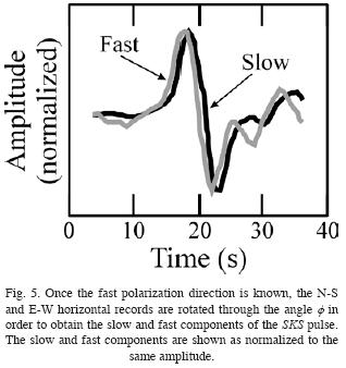
It is important to run a number of checks in order to make sure that the observation of SKS energy on the transverse component is indeed the result of anisotropy and does not arise from a different process such as scattering (Silver and Chan, 1991; Savage, 1999). Likewise, these checks mean that the values determined for Φ and δt are reliable. (1) An "unsplitting" correction is applied to the radial and transverse records using the estimated splitting parameters. If (Φ, δt) do describe anisotropy, then the SKS wave must disappear, or at least its amplitude is decreased, from the corrected transverse component (Fig. 2). Similarly, the amplitude of SKS is increased on the corrected radial component, although this is a small effect. (2) The particle motion of SKS in the transverse component is plotted as function of particle motion in the radial component. Before the unsplitting correction, particle motion must be approximately elliptical, and after correction it becomes linear (Fig. 4). (3) The N–S and E–W records are rotated through the angle Φ to obtain the slow and fast components of the SKS pulse. The fast and slow waveforms must have roughly the same shape and the fast SKS must arrive before the slow SKS by an amount approximately equal to the measured δt (Fig. 5). Shifting the slow wave by a time ot should align it with the fast wave.

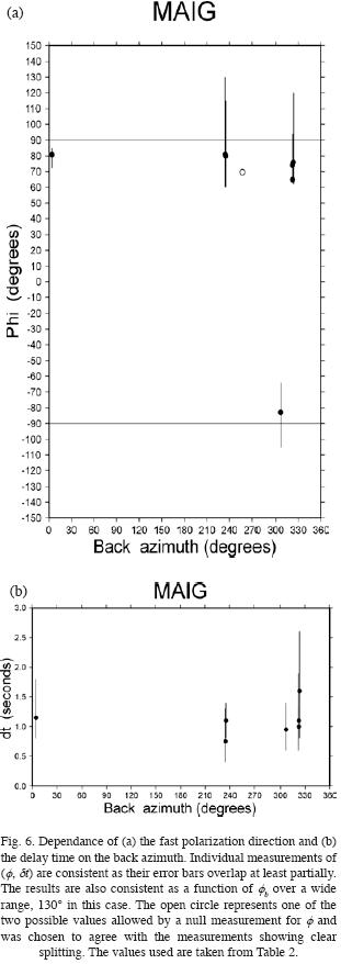
Following Silver and Chan (1991), all the individual measurements for a given station were plotted as a function of Φ_b. Fig. 6 shows the plot for station MAIG. The closed circles represent constrained measurements and the accompanying bars are their 1σ uncertainties. The latter were taken from the individual contour plots. As shown in Fig. 3, they are not necessarily symmetric. Null measurements were plotted with Φ corresponding to Φ_b or Φ_b + 90°, whichever is closer to the well constrained observations (Silver and Chan, 1991). In Fig. 6a the open circle indicates a null measurement. In this particular case, Φ= 70° and Φ_b = 257.09°. Because of symmetry considerations, Φ=70° and Φ = 70° + 180° = 250° represent the same azimuth. Consequently, Φ_b –φ = 7.09°, which means that Φ Φ_b and so the fast polarization direction is roughly oriented with the back azimuth (Silver and Chan, 1991). Values of Φ within 10–15° of the incoming polarization direction produce null measurements (Savage, 1999). The value of Φ from the null measurement is consistent with the well constrained measurements as it falls within their error bars. The delay time is plotted as a function of back azimuth in Fig. 6b. Null measurements for δt cannot be plotted. Fig. 6 also shows that individual measurements of (Φ, δt) are consistent between themselves as their error bars overlap at least partially. It can also be seen that the results are consistent as a function of Φ_b over a wide range, 130° in this example. A good coverage is desirable since it allows detecting possible azimuthal dependance of the splitting parameters which can be expected because the seismic ray path through the upper mantle is not perfectly vertical. Strong azimuthal dependance suggests that the sampled structure is more complex than one homogeneous anisotropic layer with horizontal fast and slow directions, e. g. two different anisotropic layers (Silver and Savage, 1994; Özalaybey and Savage, 1995).

 

Results

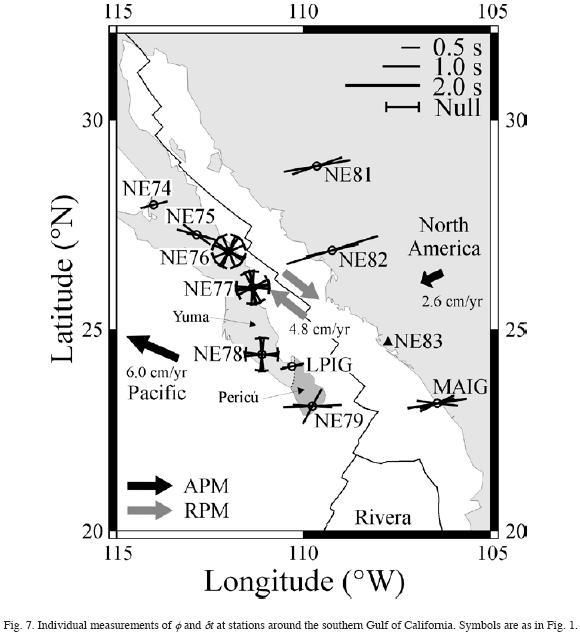
Table 1 lists the events that provided useful data for this study. Earthquake information includes the date, origin time, hypocenter, magnitude, and the geographic location. A total of 41 individual splitting measurements were made at ten different stations and are given in Table 2. The parameters are the fast polarization direction and the delay time, both with their corresponding 1 o uncertainties. Also provided are the date of the event, the back azimuth, and the phase used (SKS, SKKS, sSKS, or PKS). The observed orientations of the fast polarization direction practically span the whole space of possible solutions, from –90 to 90°. The smallest 1σ_Φ uncertainty for the fast polarization direction is 7°, while the largest is 77°. The average uncertainty is 32°. The smallest delay time is 0.55 s and the largest is 2.55 s, which may be an extreme value. The second largest delay time is 1.80 s. The average delay time is 1.12 s. The smallest 1σ_δt uncertainties for the delay time are 0.30 s, and the largest is 3.90 s at station LPIG. The second largest 1σ_δt uncertainty is 1.95 s. The average uncertainty is 0.85 s. The station with the largest number of observations is MAIG with seven records showing clearly split waveforms and one null measurement. This station had the largest number of records meeting the selection criteria previously explained. Even though records from 239 different earthquakes were available, only 23 of them generated observable P to S CMB conversions. No useful measurements could be made at station NE83. Background noise at this station, likely caused by the ocean, is particularly strong at periods between 6 and 8 s and is thus difficult to filter out given that SKS waves have most of their energy at periods from 5 to 15 s. Persaud et al., (2007) also worked with the NARS–Baja California data set. They determined crustal structure using receiver functions. In their case, NE83 was the station with the fewest useful records. Only null measurements were obtained from the three adjacent stations NE76, NE77, and NE78. Nonetheless, this is important information because it helps to narrow down the possible orientations of the fast axis, or it may indicate the absence of detectable anisotropy beneath those stations (Silver and Chan, 1991). The individual splitting parameters are shown in Fig. 7.

Average splitting parameters were calculated for each station using the stacking method of Wolfe and Silver (1998). The error surface associated to the contour plot of each individual measurement is normalized by its minimum eigenvalue, λ_2,1^min. The normalized error surfaces from all measurements at the station are then summed. In this way, the best splitting parameters are given by the minimum value of the sum and a new 95% confidence interval is obtained. As the noise properties vary for different earthquakes, stacking events with a similar polarization improves the final result (Wolfe and Silver, 1998). Therefore, the size of the 95% confidence region for the averaged values is smaller than for the individual measurements. The averaged splitting parameters are presented in Table 3, which includes the fast polarization direction and the delay time, both with their corresponding lcruncertainties, as well as the stations' coordinates and geographic location, and the total number of clearly split and null measurements. In this case, the smallest 1σ_φ uncertainties for the fast polarization direction are 5°, while the largest is 40°. The average uncertainty is 15°. The smallest delay time is 0.50 s and the largest is 2.00 s. The average delay time is 1.10 s. The smallest1σ_δt uncertainties for the delay time are 0.20 s, while the largest is 1.10 s. The average uncertainty is 0.46 s. The averaged splitting parameters are shown in Fig. 1.

The stacked average for station NE75 was calculated using only three individual measurements because the fast polarization direction for the fourth event did not fall within the 95% confidence region for the other three values. The back azimuth of the fourth earthquake is somewhat different from the others. Therefore, the anisotropy of the region it samples may be different. Additionally, two null measurements are consistent with the three observations that were stacked. For station NE82 we obtained two measurements showing clear splitting and three null measurements. The back azimuths were different for these five events. Two of the null measurements allow for a fast polarization direction which falls within the 95% confidence regions of the two clearly split measurements. Consequently, we believe that the value of Φ at NE82 is well constrained. Furthermore, the fast polarization direction for NE82 is consistent with values measured at stations NE81 and MAIG, to the north and to the south, respectively. On the other hand, the 95% confidence intervals for the two delay time measurements available at NE82 do not overlap. For this reason, the arithmetic mean of the two individual measurements for φ and δt is shown in Table 3, instead of using the stacking method of Wolfe and Silver (1998).

 

Anisotropy in the Western Mexican Basin and Range

Stations NE81, NE82, NE83, and MAIG are located in the Western Mexican Basin and Range (WMBR), which is an extensional province bounded to the east by the Sierra Madre Occidental (Sedlock et al., 1993). The WMBR is the southern continuation of the Basin and Range province of the southwestern United States (Sedlock et al., 1993).

The fast polarization direction determined at stations NE81, NE82 and MAIG is oriented approximately ENE–WSW (Fig. 1 and Table 3). No useful measurements could be made at NE83. This direction is consistent with the absolute plate motion (APM) for North America, which is oriented N244°E (Gripp and Gordon, 2002); see Fig. 1. Stations NE80 and HERB are located northwest of NE81 and their fast polarization directions are also oriented roughly ENE–WSW (Obrebski, 2007), thereby extending the region of similarly oriented fast axes from Caborca (NE80) in the northwest to Mazatlán (MAIG) in the southeast. Farther north, in the American state of Arizona, Ruppert (1992) obtained anisotropy measurements from two stations in the Southern Basin and Range (SBR) showing a fast polarization direction also oriented approximately ENE–WSW. Later work in the SBR reported the observation of Φ at three additional stations with an orientation roughly NE–SW (COARSE deployment, http://asuarray.asu.edu/coarse/images/figures/pdf/sws.pdf, 2004; Frassetto et al., 2006). Work with USArray's Transportable Array has shown further variations in the orientation of the fast polarization direction within the SBR ranging from ENE–WSW to N–S (Fouch and Gilbert, 2007). The current fast polarization direction observed in the WMBR also agrees with the extension direction for the region during the Miocene (Sedlock et al., 1993 and references therein). In the latest Miocene, the least principal stress and extension directions changed from ENE–WSW to roughly NW–SE, coeval with the initiation of rifting along the axis of the modern Gulf of California (Sedlock et al., 1993 and references therein).

Zhang et al., (2007) carried out a surface wave tomography study in the region of, and around, the Gulf of California using data from the NARS–Baja California array. The phase velocities for Rayleigh waves at periods of 10 and 14 s in the WMBR are relatively high and thus indicate the existence of thin continental crust. A thin crust is consistent with the extensional regime in the area. They also obtained fast azimuthal anisotropy directions which are approximately ENE–WSW at 10 s period, and E–W at 14 s period. The fast anisotropic axes determined from surface wave data at this depth agree reasonably well with the fast axes determined from SKS splitting. The anisotropic component from surface waves at longer periods, from 30 to 100 s (depths from 50 to 170 km), is actually small for this region (Zhang et al., 2007). Determinations of crustal thickness using receiver functions give 28 km under NE81, 26 km under NE82, and 20 km under NE83 (Persaud et al., 2007). Obrebski (2007) estimated a Moho depth of 31 km under NE81, also from receiver functions. The crustal thickness under MAIG, as determined from receiver functions, is 24 km (V. H. Espíndola, Universidad Nacional Autónoma de México, personal communication, 2007). Both kinds of data, surface waves and receiver functions, agree in showing the existence of thin continental crust, and likely thin lithosphere as well, under the WMBR. Observed delay times for stations in this region range from 0.95 to 2.00 s (Table 3). Assuming the commonly used value of 4% for shear wave anisotropy (Silver and Chan, 1991; Savage, 1999), a delay time of 1 s corresponds to an effective thickness for the anisotropic layer of 115 km. This is equivalent to anisotropic layer thicknesses ranging from 110 to 230 km, clearly thicker than the continental crust and likely thicker than the lithosphere as well. The anisotropy observed under the Western Mexican Basin and Range can thus be explained by (1) the absolute motion of the North American plate. As the thin and rigid lithosphere moves, it drags the asthenosphere underneath thereby aligning the olivine crystals in the upper mantle (Silver, 1996). Ruppert (1992) proposed that the current plate motion could explain his anisotropy observations in the SBR at mantle depths between 50 and 130 km. (2) Fossil anisotropy preserved since the Miocene at shallow depths. Fossil anisotropy has also been proposed as an explanation in the Northern Basin and Range (Great Basin) as a consequence of extension which started 30 Ma, in spite of present–day extension occurring in a different direction (Savage et al., 1990). In that case, the earlier episode of extension was larger than the modern one (Savage et al., 1990). Both possibilities are mutually compatible and suggest that the observed anisotropy in the WMBR is coherent in both the lithosphere and the asthenosphere.

 

Anisotropy in the southern Baja California peninsula

Table 3 and Fig. 1 show that, in general, the delay times measured at stations in the southern Baja California peninsula are small. Stations NE74, NE75 and LPIG have values for δt ranging from 0.50 to 0.75 s, which are near the detection threshold, i. e. δt 0.5 s (Silver and Chan, 1991). Station NE76 is interpreted to have little or no anisotropy, i. e. splitting is below the threshold of the data. Stations NE77 and NE78 either have little or no anisotropy or else their anisotropy parameters could not be measured because of the back azimuth of the incoming waves. In the latter case, their Φ axes could be oriented roughly N–S or E–W. Only station NE79, in the southernmost tip of the peninsula, has a large delay time (δt = 1.30 s) and its fast axis is oriented nearly E–W. The observation of small delays stands in contrast to the northern Baja California peninsula, where 0.70 < δt< 2.20 s as determined using data from both temporary and permanent stations (Obrebski et al., 2006; Obrebski, 2007). The fast polarization direction at many of these stations is consistently oriented E–W (Obrebski et al., 2006; Obrebski, 2007). Asthenospheric flow produced by the subduction of the Farallón plate has been proposed as an explanation for the E–W direction of the fast polarization axes under these stations (Obrebski et al., 2006; Obrebski, 2007). Likewise, the anisotropic characteristics under NE79 are also consistent with asthenospheric flow related to subduction of the Farallón plate.

Differences between the northern and the southern part of the peninsula are also clearly seen in the phase velocity work by Zhang et al., (2007). This contrast is observed in both the velocity structure and the anisotropy pattern for waves at different periods and is particularly striking at periods ranging from 50 to 80 s (depths between 50 and 150 km). At these depths the phase velocities are relatively high at latitudes roughly between 24 and 28°N. Zhang et al., (2007) propose that the high velocities are associated with the remnants of the stalled Guadalupe and Magdalena microplates which ceased to subduct 12 Ma ago. This region of high velocities agrees remarkably well with our observations of small delay times (Table 3). Low velocities (Zhang et al., 2007) are observed under the northern part of the peninsula and also south of 24°N, coincident with the location of NE79. Both regions of low velocities agree with the distribution of large delay times throughout the peninsula. Zhang et al., (2007) point out that the low velocities under the northern peninsula match the area of the slab window created during subduction of the Farallon plate. Differences between the north and the south are also observed in the pattern of azimuthal anisotropy (Zhang et al., 2007) and are particularly interesting at periods between 80 and 100s (depths greater than 150 km). The surface wave fast–propagation ani–sotropic directions are oriented E–W under the northern Baja California peninsula and have the same orientation as the shear wave splitting results (Obrebski et al., 2006; Obrebski, 2007; Zhang et al., 2007). On the other hand, surface wave anisotropy under the southern part of the peninsula at the same periods is small (Zhang et al., 2007), in agreement with the SKS observations in this study.

The differences observed between north and south peninsular seismic velocity structure are controlled by different subduction histories. The evolution of the northern Baja California peninsula is associated to the subduction of the Farallón plate (the present–day Pacific plate) and the formation of a slab window, while the evolution of the southern part of the peninsula is related to the Guadalupe and Magdalena microplates (Bohannon and Parsons, 1995). These are young slab remnants and they were difficult to subduct. Subduction of the Magdalena microplate produced arc magmatism between 24 and 12.5 Ma (Sedlock et al., 1993; Sedlock, 2003; Fletcher et al., 2007) in the region where stations with small or no anisotropy such as NE76, NE77 and LPIG are located. This is known as the Comondú Formation (Morán–Zenteno, 1994) or La Giganta volcanic belt (Ortega–Gutiérrez et al., 1992) and belongs within the Yuma tectonostratigraphic terrane (Sedlock et al., 1993). Station NE79 is located farther south and has a larger value for δt. It was unaffected by this volcanic episode and is located within the "La Paz plutonic complex" (Ortega–Gutiérrez et al., 1992), which is also identified with the Pericú terrane (Sedlock et al., 1993). By 12.5 Ma, the North American continent moved west and the volcanic arc became positioned over the thermal anomaly of the former Magdalena ridge, previously located to the west, causing asthenospheric upwelling through the Magdalena slab which had broken (Fletcher et al., 2007). Vertical upwelling may explain the small delay times observed because SKS splitting measurements are only sensitive to fast axes oriented horizontally. In certain regions around the world little splitting has been found for any polarization direction (Savage, 1999). These locations are candidates for possible near–vertical orientation of a axes (Savage, 1999). Examples include the Rocky Mountains (Savage et al., 1996), the Pakistan Himalayas (Sandvol et al., 1994, 1997), and Australia (Clitheroe and Van der Hilst, 1998).

Considering the preceding discussion, the small delay times observed throughout most of the southern Baja California peninsula may be explained by (1) the anisotropic (or isotropic) characteristics of the subducted fragments of the Guadalupe and Magdalena microplates observed (Zhang et al., 2007) under most of the southern peninsula. (2) A complex velocity structure under the stations which changes as a function of depth and thus cancels out any anisotropy accrued throughout the upgoing SKS path. (3) Vertical mantle upwelling produced as a consequence of the plate reorganization as ritfing initiated along the axis of the modern Gulf of California. Shear wave splitting measurements of SKS are only sensitive when the fast polarization directions are oriented horizontally.

Under station NE75 the orientation of the fast axis is WNW–ESE. This direction contrasts with the E–W fast direction obtained at stations in the northern half of the peninsula (Obrebski et al., 2006; Obrebski, 2007) and the absence of detectable anisotropy to the south under stations NE76 to NE78. As discussed by Obrebski (2007), the geometry of the subducting microplates may account for these observations. A large amount of the now extinct Farallon plate may have stalled beneath the former continental borderland when subduction stopped during the middle Miocene (Bohannon and Parsons, 1995). Several geophysical studies have provided evidence for the presence of the oceanic slab beneath the crust of the Baja California peninsula close to (Romo et al., 2001) and beneath NE75 (Persaud et al., 2007; Obrebski and Castro, 2008). At the time when subduction stopped (12.5 Ma) NE75 was located over the southern tip of the Guadalupe microplate, which used to subduct older lithosphere than the Magdalena microplate to the south (Bohannon and Parsons, 1995; Fletcher et al., 2007) and thus would have plunged somewhat more steeply. Consequently, NE75 seems to stand above a E–W trending discontinuity in the slab inclination which may be steeper to the north. This feature at upper mantle depths may account for the perturbation of asthenospheric flow revealed by the variation of the anisotropic pattern around this station. The E–W fast directions observed at stations north of NE75 could be related to fabric induced by fossil subduction (Obrebski and Castro, 2008) whereas the rotation of the fast direction toward that of the Pacific Plate motion at NE75 and the absence of coherent anisotropy south of it may be an effect of the northwestward motion of the relatively steep trailing Guadalupe slab along with the Pacific–Baja California plate (Obrebski, 2007).

 

Conclusions

Shear wave splitting parameters of upper mantle anisotropy under stations around the southern Gulf of California can be divided into two regions: the southern half of the Baja California peninsula and the Western Mexican Basin and Range province. In the WMBR the fast polarization direction is oriented ENE–WSW and the delay times range from 0.95 to 2.00 s, equivalent to anisotropic layers varying in thickness from 110 to 230 km. The observations can be explained by the absolute motion of the North American plate and imply that the lithosphere, presumably thin, drags the asthenosphere underneath thus aligning the mantle minerals and creating the anisotropy. Additionally, the extensional episode that affected this region during the Miocene, prior to the opening of the Gulf of California, is recorded in the form of fossil anisotropy oriented in the same direction as the asthenospheric anisotropy. These observations are consistent with results from the Basin and Range north of the area chosen for this study. Across the gulf, in the southern Baja California peninsula, small delay times are observed. These vary from 0.50 to 0.75 s, corresponding to anisotropic layers ranging in thickness between 60 and 85 km. Station NE76 is considered to have splitting below the threshold of the data, i. e. little or no anisotropy. Stations NE77 and NE78 could also have splitting below the threshold of the data, or else the fast polarization direction may be aligned N–S or E–W. These measurements stand in contrast to the larger delay times, many of them oriented E–W, observed in the northern peninsula and which have been associated to asthenospheric flow in response to subduction of the Farallon slab. The only exception to small delays occurs under station NE79 in the southernmost tip of the peninsula. The delay time is 1.30 s and the anisotropic layer is 150 km thick. The fast axis is aligned E–W. In this case anisotropy may be explained by mantle flow associated to the subduction of the Farallon plate. The anisotropic nature under the peninsula, as determined from splitting observations, seems consistent with surface wave data at periods between 80 and 100 s (Zhang et al., 2007). At these periods, the fast–propagation anisotropic directions are oriented E–W under the northern peninsula and anisotropy is small under the southern peninsula. The small splitting values observed in the southern part of the peninsula may be explained by the subducted fragments of the Guadalupe and Magdalena microplates. Alternatively, they could be explained by mantle upwelling of hot material from the former Magdalena ridge through a break in the subducted Magdalena slab. Station NE75 appears to be located at the transition between the northern region of E–W fast directions associated with fossil subduction–induced fabric, and the southern region where anisotropy is small. In any case, the history, geometry and age of subduction at the former Baja California trench seem to control the characteristics of the observed anisotropy throughout the peninsula.

 

Acknowledgments

We are thankful to Karen Fischer for providing the computer code to measure the splitting parameters; Luis Fernando Terán for the computer code to check the measurements; Manuel Velásquez for computer support; Hanneke Paulssen, Karen Fischer, Arie van der Berg, Renate den Hartog, Vlad Manea, Rob Govers, John Fletcher, and Luca Ferrari for discussions and suggestions. The suggestions made by Cinna Lomnitz, Javier Pacheco, Satoshi Kaneshima, and Takeshi Mikumo helped improve the manuscript. John Fletcher, Hanneke Pauls sen, and Xyoli Pérez–Campos provided manuscripts ahead of publication. The operation and data acquisition from the NARS–Baja California array has been possible due to the work by Arturo Pérez–Vertti, Arie van Wettum, Robert Clayton, Jeannot Trampert, and Cecilio Rebollar. We also acknowledge the participation of Antonio Mendoza, Luis Inzunza, Jeroen Ritsema, and Hanneke Paulssen. The operation and data acquisition from Mexico's Servicio Sismológico Nacional broadband network has been possible due to the work by Javier Pacheco, Carlos Valdés, Shri Krishna Singh, Arturo Cárdenas, José Luis Cruz, Jorge Estrada, Jesús Pérez, and José Antonio Santiago. One of us (SACvB) received partial funding from the Molengraaff Fonds and Trajectum Beurs for travel to and living expenses while in Mexico. This work was funded by Mexico's Consejo Nacional de Ciencia y Tecnología through grant 34299–T. The contour plots and some maps in this study were made using the Generic Mapping Tools (GMT) package (Wessel and Smith, 1998).

 

Bibliography

Anderson, M. L., G. Zandt, E. Triep, M. Fouch and S. Beck, 2004. Anisotropy and mantle flow in the Chile–Argentina subduction zone from shear wave splitting analysis. Geophys. Res. Lett., 31, L23608, doi: 10.1029/2004GL020906.        [ Links ]

Barruol, G., P. G. Silver and A. Vauchez, 1997. Seismic anisotropy in the eastern United States: Deep structure of a complex continental plate. J. Geophys. Res., 102, 8329–8348.        [ Links ]

Bohannon, R. G. and T. Parsons, 1995. Tectonic implications of post–30 Ma Pacific and North American relative plate motions. Geol. Soc. Am. Bull., 107, 937–959.        [ Links ]

Clayton, R. W., J. Trampert, C. Rebollar, J. Ritsema, P. Persaud, H. Paulssen, X. Perez–campos, A. Van Wettum, A. Perez–vertti and F. Diluccio, 2004. The NARS–Baja seismic array in the Gulf of California rift zone. MARGINS Newsletter, 13, 1–4.        [ Links ]

Clitheroe, G. and R. Van Der Hilst, 1998. Complex anisotropy in the Australian lithosphere from shear–wave splitting in broadband SKS records, in Structure and evolution of the Australian continent, Geodyn. Ser., Vol. 26, edited by J. Braun et al., 73–78, American Geophysical Union, Washington, D. C.        [ Links ]

Crampin, S and J. H. Lovell, 1991. A decade of shear–wave splitting in the Earth's crust: What does it mean? What use can we make of it? And what should we do next? Geophys. J. Int., 107, 387–407.        [ Links ]

Fischer, K. M., E. M. Parmentier, A. R. Stine and E. R. Wolf, 2000. Modeling anisotropy and plate–driven flow in the Tonga subduction zone back arc. J. Geophys. Res., 105, 16,181–16,191.        [ Links ]

Fletcher, J. M., M. Grove, D. Kimbrough, O. Lovera and G. E. Gehrels, 2007. Ridge–trench interactions and the Neogene tectonic evolution of the Magdalena shelf and southern Gulf of California: Insights from detrital zircon U–Pb ages from the Magdalena fan and adjacent areas. Geol. Soc. Am. Bull., 119, 1313–1336.        [ Links ]

Forsyth, D. W., 1975. The early structural evolution and anisotropy of the oceanic upper–mantle. Geophys. J. R. astr. Soc., 43, 103–162.        [ Links ]

Fouch, M. J., K. M. Fischer, E. M. Parmentier, M. E. Wysession and T. J. Clarke, 2000. Shear wave splitting, continental keels, and patterns of mantle flow. J. Geophys. Res., 105, 6255–6275.        [ Links ]

Fouch, M. J. and H. J. Gilbert, 2007. Complex upper mantle seismic structure across the southern Colorado Plateau/Basin and Range I: Results from shear wave splitting analysis (abstract). Eos Trans. AGU, 88 (52), Fall. Meet. Suppl., Abstract S41B–0557.        [ Links ]

Frassetto, A., H. Gilbert, G. Zandt, S. Beck and M. J. Fouch, 2006. Support of high elevation in the southern Basin and Range based on the composition and architecture of the crust in the Basin and Range and Colorado Plateau. Earth Planet. Sci. Lett., 249, 62–73.        [ Links ]

Gripp, A. E and R. G. Gordon, 2002. Young tracks of hotspots and current plate velocities. Geophys. J. Int., 150, 321–361.        [ Links ]

Hall, C. E., K. M. Fischer, E. M. Parmentier and D. K. Blackman, 2000. The influence of plate motions on three–dimensional back arc mantle flow and shear wave splitting. J. Geophys. Res., 105, 28,009–28,033.        [ Links ]

Hess, H. H., 1964. Seismic anisotropy of the uppermost mantle under oceans. Nature, 203, 629–631.        [ Links ]

Lay, T. and C. J. Young, 1991. Analysis of seismic SV waves in the core's penumbra. Geophys. Res. Lett., 18, 1373–1376.        [ Links ]

Mcnamara, D. E., T. J. Owens, P. G. Silver and F. T. Wu, 1994. Shear Wave Anisotropy Beneath the Tibetan Plateau. J. Geophys. Res., 99, 13,655–13,665.        [ Links ]

Montagner, J.–P. and T. Tanimoto, 1990. Global anisotropy in the upper mantle inferred from the regionalization of phase velocities. J. Geophys. Res., 95, 4797–4819.        [ Links ]

Moran–zenteno, D., 1994. Geology of the Mexican Republic. The American Association of Petroleum Geologists, AAPG Studies in Geology 39, 160 pp., Tulsa, Oklahoma.        [ Links ]

Nicolas, A. and N. I. Christensen, 1987. Formation of anisotropy in upper mantle peridotites – A review, in Composition, structure and dynamics of the lithosphere–asthenosphere system, Vol. 16, edited by K. Fuchs and C. Froidevaux, 111–123, American Geophysical Union, Washington, D. C.        [ Links ]

Obrebski, M. J., 2007. Estudio de la anisotropía sísmica y su relación con la tectónica de Baja California. Ph. D. thesis, 221 pp., Centro de Investigación Científica y de Educación Superior de Ensenada, Ensenada, Baja California, Mexico.        [ Links ]

Obrebski, M. and R. R. Castro, 2008. Seismic anisotropy in northern and central Gulf of California region, Mexico, from teleseismic receiver functions and new evidence of possible plate capture. J. Geophys. res., 113, B03301, doi: 10.1029/2007JB005156.        [ Links ]

Obrebski, M., R. R. Castro, R. W. Valenzuela, S. Van Benthem and C. J. Rebollar, 2006. Shear–wave splitting observations at the regions of northern Baja California and southern Basin and Range in Mexico. Geophys. Res. Lett., 33, L05302, doi:10.1029/2005GL024720.        [ Links ]

Ortega–Gutierrez F., L. M. Mitre–salazar, J. Roldan–Quintana, J. Aranda–gomez, D. Moran–zenteno, S. Alaniz–Alvarez and A. Nieto–Samaniego, 1992. Carta geológica de la República Mexicana, Fifth edition, scale 1:2,000,000, Instituto de Geología, Universidad Nacional Autónoma de México, Mexico City, Mexico.        [ Links ]

Özalaybey, S. and M. K. Savage, 1995. Shear–wave splitting beneath western United States in relation to plate tectonics. J. Geophys. Res., 100, 18,135–18,149.        [ Links ]

Peng, X. and E. D. Humphreys, 1997. Moho dip and crustal anisotropy in northwestern Nevada from teleseismic receiver functions. Bull. Seism. Soc. Am., 87, 745–754.        [ Links ]

Persaud, P., X. Perez–Campos and R. W. Clayton, 2007. Crustal thickness variations in the margins of the Gulf of California from receiver functions. Geophys. J. Int., 170, 687–699.        [ Links ]

Peyton, V., V. Levin, J. Park, M. Brandon, J. Lees, E. Gordeev and A. Ozerov, 2001. Mantle flow at a slab edge: Seismic anisotropy in the Kamchatka region Geophys. Res. Lett., 28, 379–382.        [ Links ]

Raitt, R. W., G. G. Shor, T. J. G. Francis and G. B. Morris, 1969. Anisotropy of the Pacific upper mantle. J. Geophys. Res., 74, 3095–3109.        [ Links ]

Romo, J. M., J. Garcia–Abdeslem, E. Gomez–Treviño, F. J. Esparza and C. Flores, 2001. Resultados preliminares de un perfil geofísico a través del desierto de Vizcaíno en Baja California Sur, México (in Spanish). Geos Boletín Informativo de la UGM, 21, 96–107.        [ Links ]

Ruppert, S. D., 1992. Tectonics of western North America. A teleseismic view. Ph. D: thesis, 216 pp., Stanford University, Stanford, California.        [ Links ]

Sandvol, E., J. F. Ni, T. M. Hearn and S. Roecker, 1994. Seismic azimuthal anisotropy beneath the Pakistan Himalayas. Geophys. Res. Lett., 21, 1635–1638.        [ Links ]

Sandvol, E., J. Ni, R. Kind and W. Zhao, 1997. Seismic anisotropy beneath the southern Himalayas–Tibet collision zone. J. Geophys. Res., 102, 17,813–17,823.        [ Links ]

Savage, M. K., 1999. Seismic anisotropy and mantle deformation: What have we learned from shear wave splitting? Rev. Geophys., 37, 65–106.        [ Links ]

Savage, M., J. Park and H. Todd, 2007. Velocity and anisotropy structure at the Hikurangi subduction mar gin, New Zeal and from receiver functions. Geophys. J. Int., 168, doi:10.1111/j.1365–246X.2006.03086.x.        [ Links ]

Savage, M. K., A. F. Sheehan and A. Lerner–lam, 1996. Shear–wave splitting across the Rocky Mountain Front. Geophys. Res. Lett., 23, 2267–2270.        [ Links ]

Savage, M. K., P. G. Silver and R. P. Meyer, 1990. Observations of teleseismic shear–wave splitting in the Basin and Range from portable and permanent stations. Geophys. Res. Lett., 17, 21–24.        [ Links ]

Sedlock, 2003. Geology of the Baja California peninsula and adjacent areas. 1–42, Geological Society of America, Special Paper 374, Boulder, Colorado.        [ Links ]

Sedlock, R. L., F. Ortega–Gutierrez and R. C. Speed, 1993. Tectonostratigraphic terranes and tectonic evolution of Mexico. Geological Society of America, Special Paper 278, 146 pp., Boulder, Colorado.        [ Links ]

Silver, P. G., 1996. Seismic anisotropy beneath the continents: Probing the depths of Geology, Annu. Rev. Earth Planet. Sci., 24, 385–432.        [ Links ]

Silver, P. G. and W. W. Chan, 1988. Implications for continental structure and evolution from seismic anisotropy. Nature, 335, 34–39.        [ Links ]

Silver, P. G. And W. W. Chan, 1991. Shear wave splitting and subcontinental mantle deformation. J. Geophys. Res., 96, 16,429–16,454.        [ Links ]

Silver, P. G. and S. Kaneshima, 1993. Constraints on mantle anisotropy beneath Precambrian North America from a transportable teleseismic experiment. Geophys. Res. Lett., 20, 1127–1130.        [ Links ]

Silver, P. G. and M. K. Savage, 1994. The interpretation of shear–wave splitting parameters in the presence of two anisotropic layers. Geophys. J. Int., 119, 949–963.        [ Links ]

Singh, S. K., J. Pacheco, F. Courboulex and D. A. Novelo, 1997. Source parameters of the Pinotepa Nacional, Mexico, earthquake of 27 March, 1996 (Mw = 5.4) estimated from near–field recordings of a single station. J. Seismol., 1, 39–45.        [ Links ]

Trampert, J., H. Paulssen, A. Van Wettum, J. Ritsema, R. Clayton, R. Castro, C. Rebollar and A. Perez–Vertti, 2003. New array monitors seismic activity near the Gulf of California in Mexico. Eos Trans. AGU, 84, 29, 32.        [ Links ]

Valdes Gonzalez, C., A. Cardenas Ramirez, J. L. Cruz Cervantes, J. Estrada Castillo, J. Perez Santana, J. A. Santiago Santiago, C. Jimenez Cruz, A. Gutierrez Garcia and B. Rubi Zavala, 2005. ¿20 años después del sismo de 1985, sísmicamente qué le falta a la red del Servicio Sismológico Nacional? (abstract). Geos Boletín Informativo de la UGM, 25 (1), 185.        [ Links ]

Van Benthem, S. A. C, 2005. Anisotropy and flow in the uppermantle under Mexico. M. Sc. thesis, 41 pp., Utrecht University, Utrecht, The Netherlands.        [ Links ]

Vauchez, A. and G. Barruol, 1996. Shear–wave splitting in the Appalachians and the Pyrenees: Importance of the inherited tectonic fabric of the lithosphere. Phys. Earth Planet. Int., 95, 127–138.        [ Links ]

Wessel, P. and W. H. F. Smith, 1998. New, improved version of Generic Mapping Tools released. Eos Trans. AGU, 79, 579.        [ Links ]

Wolfe, C. J. and P. G. Silver, 1998. Seismic anisotropy of oceanic upper mantle: Shear wave splitting methodologies and observations. J. Geophys. Res., 103, 749–771.        [ Links ]

Wysession, M. E., K. M. Fischer, T. J. Clarke, G. I. Al–eqabi, M. J. Fouch, P. J. Shore, R. W. Valenzuela, A. Li and J. M. Zaslow, 1996. Slicing into the Earth. Eos Trans. AGU, 77, 477, 480–482.        [ Links ]

Zhang, X., H. Paulssen, S. Lebedev and T. Meier, 2007. Surface wave tomography of the Gulf of California. Geophys. Res. Lett., 34, L15305, doi:10.1029/ 2007GL030631.        [ Links ]