Articles

 

AVOA technique for fracture characterization: resolving ambiguity

 

V. Sabinin and T. Chichinina¹

 

¹ Instituto Mexicano del Petróleo. Eje Central Lázaro Cárdenas, 152, Mexico, City, Mexico. E–mail: tichqvoa@yahoo.com

 

Received: July 14, 2006
Accepted: October 25, 2007

 

Resumen

Se desarrolla una nueva técnica de cálculo en el análisis de amplitud contra distancia fuente–receptor y contra acimut (AVOA) que resuelve la ambigüedad en la estimación de las direcciones principales de fracturas. Se analiza el tercer término de la aproximación de Rüger para el coeficiente de reflexión de ondas P, para distinguir la dirección de fracturas y la dirección de simetría. La técnica se prueba con datos reales del campo y datos sintéticos.

Palabras clave: AVOA, el medio HTI, anisotropía sísmica, caracterización de yacimientos fracturados.

 

Abstract

A new computational technique of AVOA analysis (Amplitude Versus Offset and Azimuth) is developed which resolves an ambiguity in fracture–direction estimation. It analyzes a third term of Rüger's approximation for P–wave reflection coefficient to distinguish symmetry–axis and fracture–strike directions. The technique is tested on synthetic and field data.

Key words: AVOA, HTI media, seismic anisotropy, fracture–reservoir characterization.

 

Introduction

The analysis of azimuthal variation in reflection coefficients or AVOA analysis (Amplitude Versus Offset and Azimuth) is widely applied for detecting and mapping highly fractured zones with azimuthally–oriented vertical cracks. Based on the Rüger (1998) approximation for the reflection coefficients in HTI medium, the AVOA technique gives, in general, two principal symmetry directions of HTI medium without any formal indication of which of these two directions points to the symmetry axis, and which to the fracture strike. As shown by Zheng et al. (2004), some additional information is required besides the reflection coefficients to resolve the ambiguity in fracture–direction estimation.

We develop a computational technique for PP–wave AVOA analysis improved in comparison with existing techniques, which resolves the ambiguity using only information obtained from amplitudes (or reflection coefficients). The technique analyzes the third term of Rüger's approximation for determining symmetry–axis and fracture–strike azimuths uniquely. We test the algorithm on synthetic and field data.

 

Background

The methodology of AVOA analysis is based on the concept of azimuthal anisotropy caused for the most part by parallel vertical fractures. It leads to the azimuthal anisotropy of amplitudes, in particular, to azimuthal variation in reflection coefficients. The fractured reservoir is represented by a model of a transversely isotropic medium with horizontal symmetry axis (HTI medium). The FF–wave reflection coefficient R at the interface (or reflecting boundary) between weakly anisotropic HTI media (or between isotropic and HTI media) is defined by the approximate formula (Rüger, 1998):

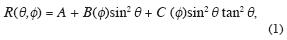
where θ is the incidence angle, and is the source–receiver–line azimuth with respect to the coordinate axis x. The term A is the normal–incidence reflection coefficient

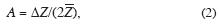
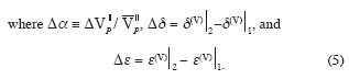
where is the vertical P–wave impedance, V_p¹¹ is the vertical velocity (or velocity in the isotropy plane) of the P wave, Δ denotes the difference between the values of a parameter below and above the reflecting boundary, and the bar ... indicates the mean of these values.

The coefficient B () is a so–called AVO gradient, which can be written (Rüger, 1998)

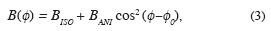
where ₀ is the angle of the symmetry axis with the x–axis. The term B_ISO is the AVO–gradient isotropic part (equal to the AVO gradient for isotropic media), and B_ANI is the anisotropic part of the AVO gradient.

The last term in equation (1), that is, the term with the coefficient C(), gives a marked contribution to the reflection coefficient value only for distant offsets (large incidence angles). The coefficient C() can be written (Rüger, 1998)

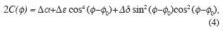
Following the terminology of Rüger (1998) and Ts–vankin (1997), the Thomsen–style anisotropy parameters ε^(v), δ^(v) and g are used to describe the anisotropy of HTI media, which are effective models of vertically fractured rocks. The parameters ε^(v), and δ^(v) are negative, γ is positive for HTI medium (Bakulin et al., 2000), and they are equal to zero for an isotropic medium. The difference in anisotropy parameters across the boundary is written with the help of Δ in (4) – (5) as above, and the subscripts |₁ and |₂ refer to the upper or lower medium respect to the boundary.

The main problem is to estimate the symmetry–axis angle ₀. The technique which we propose is based on equations (1) – (5). Note that equation (1) is intended for calculation of reflection coefficients, while in real data, one deals with amplitudes of reflected waves, not with reflection coefficients. This brings some problems. We may not use instantaneous amplitude due to its high variability. Instead, we must take into consideration some integral characteristic of a signal for imitation of amplitude. A proper definition of this integral amplitude from wave samples of seismic records is required because amplitude estimation is very sensitive to noise and errors. Depending on this definition, the sign of amplitude may sometimes differ from the sign of the reflection coefficient; therefore it is necessary to know the sign of the difference of impedances across the boundary (see equation (2)). Also, it is necessary to correct the amplitudes for geometrical spreading, which procedure is not simple or exact for anisotropic media. Our solution of these problems is presented in Appendix A.

 

Algorithm

The algorithm for estimating the symmetry axis angle ₀ may be divided into three steps. The first step consists in estimating the coefficients A, B and C in equation (1). The second step is defining two principal symmetry directions of HTI medium using the formula (3) for the AVO gradient B. The third step is analyzing the coefficient C, equation (4), to distinguish the symmetry axis direction from the fracture strike.

The first step of the algorithm is the estimation of A(), B(), and C() for each individual azimuth–sectored CMP gather. The coefficients A, B and C in equation (1) are determined by the least–squares method. For each source–to–receiver line j ( j = 1,...,n ), the functional

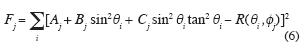
is to be minimized. Here i is the number of the offset (corresponding to the incidence angle θ_i) in the j–th azimuth–sectored CMP gather. The coefficients A, B and C are determined from the system of three linear equations

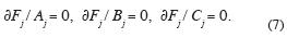
This procedure is repeated for each j (j = 1,...n ). Due to azimuthal anisotropy of the medium, the AVO gradient B acquires different values B₁ B₂, ..., B_n for n azimuth–sectored CMP gathers.

The second step of the algorithm consists in the estimation of the angle ₀ from equation (3). For this purpose, at least three AVO–gradient values are required, each of them estimated for a different source–to–receiver line azimuth (or sector). For n=3 the problem was solved by Mallik et al. (1998). For n>3 the problem is solved by the least–squares method as follows.

As the A value should not depend on azimuth, but the A values may be calculated different for different azimuths, then we should normalize the AVO gradient B as B_j / A_j = B_j , where A_j and B_j are calculated above by the least–squares method for each azimuth sector j. Formula (3) for the normalized AVO gradient can be rewritten by trigonometric transformation in the form

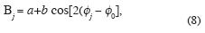
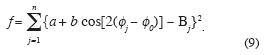
where _j is the mean azimuth of the j–th azimuth sector for real data, or the azimuth value for synthetic data. The values B = B/ A are already known as estimated in the first step. The parameters a, b, and ₀ are unknown, and can be obtained by minimizing the functional

This yields the system of equations

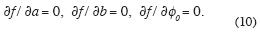
From (10), we derive an analytical trigonometric equation for ₀ (given in Appendix B) and we find that the solution ₀ has a period of 0. This value of the period means that we cannot be sure whether Φ₀ is the symmetry–axis azimuth or the orthogonal direction, i.e. the fracture–strike. Also from equations (8), one can infer two different solutions, namely (a, b, ₀) or (a, –b, ₀ ± , see also Zheng et al. (2004). These solutions are the local minima of the functional (9), as may be confirmed by evaluating the second partial derivatives of the functional f.

 

How to distinguish fracture strike from symmetry axis

For some cases, the ambiguity in fracture–orientation detection may be resolved by analyzing the AVO–gradient dependence on , equation (3). As shown by Hall & Kendall (2000), and by Zheng et al. (2004), when the sign of B_ANI is known beforehand it is possible to solve the problem. However, in general, the sign of B_ANI may be arbitrary. For many anisotropic media B_ANI > 0. But as shown by Chichinina et al. (2003), anisotropic media with B_ANI < 0 are not exotic, and one can be sure that B_ANI > 0 for a given HTI medium as long as, for host–rock velocities, the ratio V_S/V_P > 0.56 is valid.

Let us rewrite equation (4) as

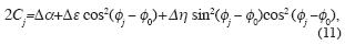
where j = 1,...,n, Δ η = Δ δ – Δ ε, and Δ ε is given by equation (5).

When substituting the value ₀ ± instead of ₀ into equation (11), the sign of the second term in the sum, Δ ε cos²(_j –₀), switches to the opposite sign, because equation (11) takes the form

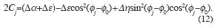
Note that Δ ε should be negative for the upper reflecting boundary of the HTI layer (the case of HTI layer overlain by an isotropic overburden), and positive for the lower reflecting boundary (i.e., for the interface HTI medium –isotropic medium). This follows from equation (5), taking into account ε^(v)= 0 in the isotropic medium and ε^(v)< 0 in the HTI medium.

Thus, the sign of Δε is predefined for the model. If, for a given ₀, the sign of Δε from equation (11) does not satisfy the condition for the boundary of HTI layer mentioned above, it means that ₀ is the fracture–strike direction, because the sign of the term Δεcos²(_j –₀) is changed. Thus, if the sign of Δε could be estimated, the ambiguity problem would be solved.

At first, we will normalize both sides of equation (11), dividing by A, as was done for equation (8), and assume from now on that C = C/ A, Δα = Δα/A_j. Δε Δε/A_j, and Δη Δη /A_j.

Then the value of the new normalized Δ ε can be estimated by minimizing the following functional f₁, using the least–squares method:

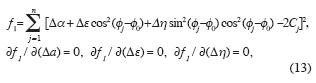
where ₀ is one of the known solutions of system (10).

The system of equations (13) is solved by analogy with the system of equations (6) – (7).

Keeping in mind the sign requirements for non–normalized Δε, we suggest the following criterion for identification of the solution ₀ as the symmetry–axis azimuth:

for upper reflecting boundary of the HTI layer

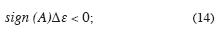
for lower reflecting boundary of the HTI layer

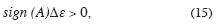
where the value of normalized Δ ε is assumed to be calculated from equations (13).

In (14) and (15), the term sign (A) is the sign of the normal–incidence reflection coefficient A, which can be determined from the impedance change over the boundary, equation (2), or from equations (7). If one deals with data of amplitudes (not with data of reflection coefficients), then one can not be certain of using sign (A) from the system of equations (7), because the sign of the amplitude might not match the sign of the reflection coefficient. For example, this might arise from distortion of wave form that could lead to a changed sign of integral amplitude (see Background, and Appendix A).

 

Examples of algorithm application

We tested the algorithm using synthetic data shown in Fig. 1, and we applied it to field data shown in Fig. 2.

Tests with synthetic data. The synthetic data are represented by three CSP seismograms corresponding to three source–to–receiver–line azimuths 0°, 45° and 90°. These synthetic seismograms were generated by the ray method (Obolentseva and Grechka, 1989). Figure 1 shows one seismogram (for the azimuth of 45°) as an illustration. The model consists of 11 layers and describes the subsurface of the Urubchen–Tokhomo Area (Eastern Siberia), in which the HTI layer is the tenth (460 m–thick Riphean carbonates). The symmetry–axis azimuth of the HTI layer is ₀ = 60°. The Thomsen parameters and density for this layer as well as vertical velocities (V^||_S, V^||_P) and density for isotropic layers above and below the HTI layer are given in Table 1.

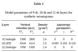
The proposed AVOA technique can be applied to the upper as well as the lower boundary of HTI layer. Here we performed AVOA analysis for the lower reflecting boundary of the HTI layer at a depth of 2665 m, and for the upper reflecting boundary of the HTI layer at a depth of 2205 m, both marked by arrows in Figure 1. Note from Table 1 a negative change of the impedance over the lower boundary, that is A < 0, and a positive change of the impedance over the upper boundary (A > 0).

For calculating the incidence angles from offsets, we used ray–tracing in the multi–layered model, or a one–layer approximation which considers the layered medium above the reflecting boundary as a homogeneous layer. The ray–tracing was performed by Snell's law using the formula (Tsvankin, 1997) V_P = V_P^||[1+δ^(v)sin²θcos²θ+ε^(v) cos⁴θ] for the velocity in the anisotropic layer, if needed.

When using the ray–tracing for calculating q, we estimated from (6) – (10) f0 = 60.53° for the upper boundary, and ₀=60.9° for the lower boundary. When using the one–layer approximation, we estimated ₀ =61.26° for the upper boundary, and ₀ = 61.26° for the lower boundary. Thus, the accuracy was better than 1.5% for the ray–tracing, and 2% for the one–layer approximation.

With a knowledge of these values of ₀, we now use the algorithm for distinguishing the symmetry–axis direction by calculating the parameter Δ ε found from (13). We obtained Δ ε < 0 for both boundaries in all considered cases, which yields sign (A)Δ ε < 0 for the upper boundary and sign (A)Δ ε > 0 for the lower boundary, as it should be for the symmetry axis, equations (14) and (15).

To simulate real data, we added a random Gaussian white noise to the synthetic seismograms. Maximum amplitude of the noise was chosen as 10%, and as 20% of the maximum amplitude of the signal reflected from the upper boundary of the HTI layer at the first trace. As the amplitudes of reflected waves in the traces decrease with offset up to 2.3 times, the actual error caused by the 20% noise was up to 45% for distant offsets.

For the upper boundary, in the case of ray tracing, we obtained ₀ = 63.64° for 10% noise, and ₀ = 64.12° for 20% noise. For the lower boundary the respective values were ₀ = 59.39° for 10% noise, and ₀ = 58.03° for 20% noise. Such a difference between the results for the boundaries can be explained by interference of the waves reflected from the upper boundary with the waves reflected from the preceding boundary (see Fig. 1), the superposition interval is equal to 10 ms. To reduce the influence of interference, an additional smoothing can be applied (see Appendix A) for obtaining better results for the upper boundary.

In the case of calculation with the one–layer approximation, the results were as follows: for the upper boundary (with additional smoothing) ₀ = 62.98° for 10% noise, and ₀ = 63.4° for 20% noise; for the lower boundary ₀ = 61.52° for 10% noise, and ₀ = 57.91° for 20% noise. The one–layer approximation seems to be a good alternative to ray–tracing for the data used.

Application to field data. The field data contain 12 seismograms from 12 azimuth sectors (Fig. 2) for a su–perbin of 13x13 bins acquired at the Vancor Area (Eastern Siberia, Russia) in 2004. The target reflection is from the top of the HTI layer (overlain by an isotropic overburden) at the depth of 3.4 km marked by an arrow in Fig. 2.

The analysis of azimuthal variation in the AVO gradient provided two principal directions of symmetry: –4.3° and 85.7° (Fig. 3). From these two directions we distinguished the azimuth of 85.7° as the symmetry–axis direction. We used our criterion taking into account that the coefficient A was negative due to negative impedance change across the reflection boundary, ΔZ < 0 (estimated from the sonic logs). We substituted the calculated values of C_j and ₀ = –4.3° into equations (13), and obtained the parameter Δ ε = –19.4. Following equation (14), the condition for the symmetry axis at the boundary "isotropic medium – HTI medium" requires sign (A)Δ ε < 0, but in this case sign(A)=–1, and therefore sign (A)Δ ε > 0. We concluded that ₀ = –4.3° was the fracture–strike direction, and the symmetry–axis azimuth was 85.7°.

 

Discussion and conclusion

We solve the problem of ambiguity by analyzing the sign of the parameter Δ ε which is a coefficient in the second term of (11) for the coefficient C at the third, high–angle, term in Ruger's equation (1). We realize that it is hard to obtain a reliable estimation of Ruger's high–angle term from real field data. However, actually only the sign and not the value of Δ ε is required for the criterion (14) – (15).

For determining the sign of Δ ε, we use equations (13), in which we take into account only sectors j with reliable values of coefficients C_j. For instance, in the above example of field data, the data at the azimuth sector of 7° (j=1) which give an unaccountably large value of C_j was omitted as shown in Figure 3, where the omitted points (from the polynomial fit as well as from the linear fit) are marked by crosses. The point was eliminated from the total of 12 points in the plot and only 11 points remained for the fit. Note that the corresponding AVO–gradient value B for the first sector, j=1, exhibits another unreliable value like the C_j –value, and should be excluded from the cos2( – ₀ ) –fitting for the variation B (₀ ) .

Following equations (1), and (6) – (7), it is obvious that the estimate of C_j is linked to the B_j –estimate. By selecting a reliable B_j –estimate, we can provide a reliable C_j–estimate. To select a reliable B_j–estimate, if necessary, we perform the linear fitting y=A+Bx (where xsin²θ), additionally to the polynomial fitting y=A + Bx + Cx², which is carried out in the first step, equations (6) – (7). Figure 3 shows the trend of the polynomial fit similar to the trend of the linear fit, that gives a difference of 11.8° in the ₀–estimate (₀ =7.5°). It seems sufficient to consider the used data as reliable.

Also, A_j–estimate demonstrates close values for reliable sectors, and extremely unlike values for unreliable sectors.

We believe that the technique is applicable to field data by using controlled reliable values of C, that are consistent with reliable values of B_j and A_j.

 

Acknowledgments

We thank NPO Enisey–Geofizika, Russia, for the field data provided, and the Institutes of Petroleum Geology and Geophysics of SB RAS, and VNIIGEOFIZIKA, Russia, for access to the synthetic seismograms.

 

Appendix A Using amplitudes instead of reflection coefficients

While the background of AVOA analysis is based on Ruger's formula for the reflection coefficient, equation (1), in real data AVOA analysis should use signal amplitudes. It is true that the signal amplitude is not equal to the reflection coefficient. Moreover, no picked instantaneous amplitude (sample) in the signal can be used because the signal changes form during propagation for many reasons. One should use an integral amplitude characteristic of the signal which adequately corresponds to the reflection coefficient. Let's call this characteristic simply by amplitude and denote it as P.

From our experiments, a simple definition of the amplitude as an extremum of samples in the time window of the signal 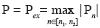, where P_n is a sample, n is a number of the sample, n₁ and n₂ are limits of the time window) was found non–satisfactory.

We found that the estimated value of ₀ is very sensitive to the definition of P, especially for data with noise. We suggest the following procedure for definition of P which gives good and stable results. The procedure calculates a maximum value of the signal envelope with a sign of the central peak of signal. In calculating the envelope, the Fourier transform of this signal is used: F = F₊+F_-, where F₊ is the part of spectrum corresponding to positive frequencies (ω>0), and F_- is the part of negative frequencies. The envelope of the signal is given by the absolute value of inverse Fourier transform of 2F₊, with F_- 0 (Sheriff & Geldart, 1983).

Limits of the signal (n₁ and n₂) are very important parameters in this definition. In the examples above, for a Ricker wavelet which has a central peak and two adjacent peaks of opposite sign, we define the time limits of the signal by including the central peak and 0.9 of the adjacent peaks. For finding the limits for data with noise, we smooth the signal by a sequence of cubic polynomials, each defined on 12 points, using the least–squares method.

For accuracy of Fast Fourier Transform one should use as many points as possible. For this, we calculate the envelope of a wave composed from the signal repeated five times, and we find the maximum from the middle part of this envelope.

Equation (1) should be rewritten for using the amplitudes. The amplitude of reflected PP–wave can be expressed as

where c_g is the coefficient of geometrical spreading (divergence) of this wave, c_g = c_g (θ ,), P_ini is the amplitude of the source (the initial amplitude), and R is the reflection coefficient R = R (θ,) in the equation (1).

The amplitude for the normal–incidence wave can be written as

where c_g0 is the normal–incidence coefficient of geometrical spreading, which does not depend on (θ,), and A is the normal–incidence reflection coefficient, A=const, equations (1) – (2). Then the reflection coefficient can be expressed as

Therefore the equation (1) for the reflection coefficient R transforms into the following equation for the amplitude P:

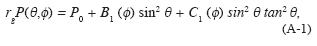
where B₁=BP₀/A, C₁=CP₀/A, and r_g c_g0 /c_g . This equation should be used in the AVOA technique instead of (1).

Note that c_g can be expressed as c_g =c_m (θ,)/r, where r is a wave path from source to receiver, and c_m depends on the direction of wave propagation (for isotropic media c_m=const). In assuming a weak anisotropy, one may assume a weak dependence of geometrical spreading on incidence angle: c_m≈ const for a given source–to–receiver line with azimuth f. Then

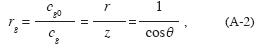
where z is the normal–incidence ray path, and c_g0 ,c_m /z. It is the approximate formula for divergent correction.

For multilayered media, the expressions for divergence correction can be found in Newman (1973). A practical methodology for the P–wave geometrical–spreading correction in layered azimuthally anisotropic media can be found in Xu & Tsvankin (2004).

 

Appendix B Formula for calculating symmetry–axis direction

There is a distribution of n B_j –values ( B₁, B₂ ,., B_n ) given for n azimuth angles _j (₁ ,₂, ..., _n). The problem is to fit the function

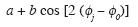
to these B_j – values (j=1, 2, ..., n).

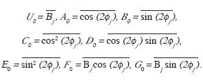
In this function, there are three unknown quantities: a, b, and ₀ which may be determined by the least–squares method, by introducing the functional f, equation (9). The goal of AVOA analysis is to determine the symmetry–axis direction, or to estimate the angle ₀. The condition for minimum of the functional f yields the system of equations (10), from which the simple trigonometric equation for ₀ is derived by excluding parameters a and b:

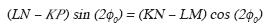
where KF₀–U₀A₀, L G₀–U₀B₀, MC₀–A₀², N D₀–A₀B₀, and P E₀–B₀², with U₀, A₀, B₀, C₀, D₀, E₀, F₀, and G₀ are determined as the arithmetic mean values (for example,

 

Bibliography

Bakulin, A., V. Grechka and I. Tsvankin, 2000. Estimation of fracture parameters from reflection seismic data – Part I: HTI model due to a single fracture set. Geophysics, 65, 1788–1802.        [ Links ]

Chichinina T., V. Sabinin and G. Ronquillo Jarrillo, 2003. Numerical modeling of P–wave AVOA in media containing vertical fractures / Expanded abstract. The Sixth International Conference on Mathematical and Numerical Aspects of Wave Propagation "Waves' 2003", Finland, Springer, 897–902.        [ Links ]

Hall, S. A. and J–M. Kendall, 2000. Constraining the interpretation of AVOA for fracture characterization: in Anisotropy 2000: Fractures, converted waves, and case studies. Soc. Expl. Geophys., 107–144.        [ Links ]

Mallik, S., K. L. Craft, L. J. Meister and R. E. Chambers, 1998. Determination of the principal directions of azimuthal anisotropy from P–wave seismic data. Geophysics, 63, 692–706.        [ Links ]

Newman, P., 1973. Divergence effects in a layered earth. Geophysics, 38, 481–488.        [ Links ]

Obolentseva, I. R. and V. Yu. Grechka, 1989. Ray method for anisotropic media (algorithms and codes). Institute of Geology and Geophysics Press, Novosibirsk, 226 p. (in Russian).        [ Links ]

Rüger, A., 1998. Variation of P–wave reflectivity with offset and azimuth in anisotropic media. Geophysics, 63, 935–947.        [ Links ]

Sheriff, R. E. and L. P. Geldart, 1983. Exploration Seismology, Volume 2, Data–processing and interpretation. Cambridge University Press, Cambridge, 400 p.        [ Links ]

Tsvankin I., 1997, Reflection moveout and parameter estimation for horizontal transverse isotropy. Geophysics, 62, 614–629.        [ Links ]

Xu, X. and I. Tsvankin, 2004. Geometrical–spreading correction for P–waves in layered azimuthally anisotropic media. 74th Ann. Internat. Mtg. Soc. of Expl. Geophys., 111–114.        [ Links ]

Zheng, Y., D. Todorovic–Marinic and G. Larson, 2004. Seismic fracture detection: ambiguity and practical solution. 74th Ann. Internat. Mtg. Soc. of Expl. Geophys., 1575–1578.        [ Links ]