Articles

 

Enhancing C2 and C3 coherency resolutions through optimizing semblance–based functions

 

Fidel Reyes–Ramos¹ and J.O. Campos–Enriquez^1,*

 

¹ Instituto de Geofísica, Universidad Nacional Autónoma de México, Del. Coyoacán, 04510 México City, México * Corresponding author: ocampos@geofisica.unam.mx Email: frramos@imp.mx

 

Received: March 13, 2007
Accepted: June 12, 2007

 

Resumen

Se calculan echados aparentes de reflectores 3–D maximizando la coherencia basada en la semblanza (C2) mediante técnicas de optimización numérica. Esta maximización fue hecha por medio de una búsqueda en una partición del dominio de los echados aparentes, y por medio de algoritmos de optimización. Se aplicaron los algoritmos simplex y Levenberg–Marquardt, cuyos desempeños fueron comparados con aquellos de las técnicas directas. De acuerdo a experimentos numéricos con datos reales, el algoritmo simplex permite no solamente importante ahorros en tiempos de cómputo, sino que proporciona también los valores más altos de la función objetivo en toda las circunstancias. Este resultado implica que el simplex realiza el proceso de maximización más eficientemente, en tanto que las otras técnicas analizadas convergen hacia la región de la solución, pero no alcanzan el máximo. Este resultado se traduce en un mejor contraste entre características coherentes y no coherentes, lo cual implica una mayor resolución. El algoritmo Levenberg–Marquardt proporciona para la coherencia los valores más pequeños. Los resultados de este estudio también encuentran aplicación en el cálculo de la coherencia normal C3 (eigenstructure). Para ello se realiza un apilamiento sesgado de las trazas de acuerdo a los echados aparentes, obtenidos previamente con la optimización de la semblanza con apilamiento sesgado C2 con la técnica simplex. La coherencia corregida por echado que se obtiene proporciona parcialmente una mejora en la resolución.

Palabras clave: Atributos sísmicos, coherencia, echados aparentes, optimización numérica

 

Abstract

Apparent dips from 3–D reflectors are calculated by maximizing the semblance–based coherency (C2) by numerical optimization techniques. This maximization was done by means of searching through a tessellation of the apparent dips domain, and by optimization algorithms. We applied the simplex and Levenberg–Marquardt, whose performance was compared with those from the direct search techniques. According to numerical experiments with real data, the simplex algorithm enables not just important computing time savings, but provides the highest values from the objective function under all circumstances. This result implies that simplex achieves the maximization process more efficiently, while the other analyzed techniques converge towards the solution region but fail attaining the maxima. This result translates into a better contrast bettween coherent and non coherent features which implies higher resolution. The Levenberg–Marquardt algorithm provides the lowest values for the coherency. These results also found application to the calculation from normal C3 coherency (eigenstructure). This is achieved by slanting the traces with the apparent dips, previously obtained by optimizing the C2 slanted semblance with the simplex technique. The obtained dip corrected coherency show partially an enhanced resolution.

Key words: Seismic attributes, coherency, apparent dips, numerical optimization

 

Introduction

Coherency is an example of complex multi trace seismic attributes. It is a measure of the similarity of traces (Neidell and Taner, 1971) and has been used in delineation of lateral changes in the seismic response due to changes in structure, stratigraphy, lithology, porosity, and the presence of hydrocarbons. An early measure of coherency was the correlation coefficient (Neidell and Taner, 1971) used to calculate seismic velocities.

The 3–D seismic coherency cube (Bahorich and Farmer, 1995, 1996) showed the potentials from the correlation–based coherency, as a seismic attribute by itself, in seismic interpretation. In particular it enabled the calculation of dip and azimuth of seismic reflectors.

The 3–D coherency cube represented an innovation at the time it was proposed. It is quite useful in delineating seismic faults and delineating subtle changes in stratigraphy (i.e., meandering distributary channels, point bars, canyons, slumps, and tidal drainage patterns). However, it was soon realized after its introduction that applied to data with low signal to noise ratio, the coherence cube was not robust.

Because of this, Marfurt et al. (1998) used the semblance as a generalized measure of coherency based in the idea of shifting in time the traces in proportion to the estimated apparent dips (slant stack). This process has been also known as Radon transform. Because of its improved robustness, the scope of its application has been widened. Marfurt et al. (1998) lists advantages of 3–D seismic coherency cubes over hand–picked horizon dip/azimuth and shaded relief maps.

The slanted semblance is estimated by:

Where (τ, p, q) represents a planar event at time τ with p and q apparent dips in the inline and crossline directions respectively; the superscript H denotes the Hilbert transform or quadrature component of the real seismic trace u, Δx and Δy the spacing of traces in inline and crossline directions, and Δt is the temporal sampling. The vertical analysis window has a height 2w or a half–height with K=w/Δt samples. The numerator of equation (1) is the 3–D transform U (τ, p, q) of the data and is related closely to the Radon transform for 3–D dip filtering and trace interpolation:

The C2 coherency, as it has been known (Marfurt et al., 1998), corresponds to the maximum value of equation (1).

Marfurt et al. (1998) proposed to discretize the domain of equation (1) and to look for those value of the variables p and q for which the slanted semblance attains its maximum. By direct search strategies we mean different ways to achieve this discretization. With the objective of testing if these strategies can be improved, we compare them to numerical algorithms, in particular to the simplex and Levenberg–Marquardt techniques.

1.1 Eigenstructure based and dip corrected coherency

The next generation of seismic coherency measure was based on the covariance matrix (Gerztenkorn and Marfurt, 1999). In a straightforward way, with J neigbouring traces comprised in, for example, a rectangular neighborhood and a time gate [–K, K] of 2K + 1 samples, we can build data vectors of dimension J by taking the amplitude of each trace at the same time level t. The jth component of this vectors is:

Where D represents a datum in a seismic cube at time t at a corresponding inline and crossline position (x_j, y_j).

The covariance matrix of the data vectors is the average of their outer product:

The eigenvalues of matrix C are always greater than or equal to zero and the eigenstructure coherency is the ratio of the first eigenvalue to the trace of C:

If data are completely coherent, the data vectors X_t are the same and the rank of C is one. Therefore, its eigenvalues are zero but the first, and because their sum is the trace of C (Golub and van Loan, 1983), the eigenstructure will be one.

The eigenstructure is the ratio of the "energy" of data in the main direction, pointed by the first eigenvector, to the sum in its orthogonal directions which are zero in case of total coherency. When there is not coherency, the eigenstructure is a minimum value not equal to zero.

Similarly to the generalization leading from C1 to C2, eigenstructure or C3 was slanted and optimized to calculate apparent dips. Accordingly, with apparent dips p and q, the components of these data vectors are:

With the corresponding covariance matrix:

And the eigenstructure optimized by the apparent dips is:

Marfurt et al. (1999) named it C3.5 coherency. Soon C3.5 was realized that it does not provides good resolution, and suffered from the "dip saturation" phenomenon (i.e., in the presence of very steep faults, the estimated apparent dips correspond to the fault trace and not to the reflectors themselves). In this way coherence is being assigned where it really does not exist, and in the resulting image, steep faults remain hidden.

To overcome this inconvenience, Marfurt et al. (1999) proposed to smooth with a low pass filter the apparent dips calculated in neighbouring positions. With the resultant dips, seismic traces are slanted before calculating the eigenstructure. Coherence C3.6 was so formulated.

Additionally to the here summarized coherencies other measures have been proposed.

Among them, we have MUSIC–based coherency (Marfurt et al., 2000) which is also based in optimizing an objective function in terms of the dips and the Higher order statistics coherency (Lu et al., 2005).

However, excepting C3 and C3.6, in all these seismic attributes the apparent dips are obtained by maximizing the respective proposed measure of coherency. This step is very important because the reliability of the obtained dips is measured by the coherency itself (Marfurt et al., 1998).

An applications of the obtained results is given in enhancing the slanted C3 coherency described above. Instead of calculating the apparent dips by maximazing directly the C3, as in C3.5 coherency, we calculated them by maximazing equation 1 by means of the optimization algorithms, and then use them to slant the traces, to finally calculate the C3 coherency; we name this variation "dip corrected eigenstructure". Here we describe our algorithms and discuss the obtained results.

2. Optimization techniques

2.1 Direct search strategies

As already mentioned, Marfurt et al. (1998) estimates (p, q) through a straightforward search over a user–defined range of apparent dips, and proposes discretizing of the search domain by rectangular, radial, or Chinese checker tessellations at whose nodes equation (1) must be evaluated (Figure 1).The distance (Δp, Δq,) grids should be

where a and b are the half–widths of the major and minor axes of the analysis window, and f_max the Nyquist temporal frequency of the seismic data.

In this way, optimization reduces to calculate directly c(τ, p₁,q_n) over n_p x n_q discrete apparent pairs (p_l,q_m) where n = 2d_max /Δp + 1 and n_p = 2d_max /Δq + 1. The interpreter defines the maximum true dip, d_max.

The above mentioned direct search strategies are not efficient because 1) to iterate through each node from the search domain is time consuming, and 2) the tessellation can miss the pair (p,q) at which equation (1) has its true maximum, i.e., the maximum is not attained efficiently as could be done by using optimization techniques (e.g., simplex or Levenberg–Marquardt techniques), as we shall demonstrate.

2.2 Simplex algorithm

The process in the simplex algorithm is based in a polyhedron whose vertices are constituted by (n+1) points belonging to the n–dimensional parameter space where the solution is sought. The polyhedron is called simplex. At each iteration the worst evaluated point is replaced by a new one, and the algorithm can create a new simplex from the previous one. This process enables the simplex to evolve and to get away from the region around the worst point of the previous simplex. The direction in which the search proceeds is given by the value of the objective function and a series of rules. In first place, this technique calculates the centroid from all the points except the worst one. The worst point is then reflected around this centroid (Figure 2a). If the function value is "better" than the best point of the simplex in the previous evaluation, it is considered that the search has conducted the simplex to a better region from the solution space. In this case an expansion is done in the given direction (i.e., the line joining the centroid and the new point) (Figure 2b). However, if the value of the function is "worst" than at the previous worst point, it is considered that the search has conducted the simplex to a bad region from the solution space. In this case a rectification is done by way of a contraction along the search direction (Figure 2c). Finally, if the function value is better than the worst point but worst than the second worst point, this contraction is limited as in Figure 2d. The contraction is controlled by a factor β (negative for case c, and positive for case d), while the expansion is controlled by the factor y. This ingenious search algorithm was first proposed by Spendley et al. (1962), and modified by Nelder and Mead (1965). Every time a new simplex is generated the objective function is evaluated three times.

Several comparative studies indicate that the simplex algorithm is robust in the presence of noise, and Box and Draper (1969a, b) considered it as the best one from all the sequential search algorithm.

2.3 The Levenberg–Marquardt algorithm.

It is based on the family of gradient descent algorithms (i.e., Rao, 1996). In order to maximize a function of several variables, a vector of a proposed solution X_i is improved by adding to it the term –(H–λI)^–1f, where H and f are respectively the Hessian matrix and gradient of the objective function (1), I the identity matrix and λ a regularization factor. In the Levenberg Marquardt, the trace of the identity matrix is replaced with the trace of the Hessian in order to avoid the optimization process "oscillates" around a solution. If the new solution is better than the old one, the λ factor is replaced by its half, otherwise, it is doubled.

A problem with this algorithm is the inversion of matrices and this factor increases its computational cost. However, the Levenberg–Marquardt was chosen because other gradient–based techniques require that the objective function must be maximized along a parameterized line between two vectors of proposed solutions, and this increases their computational cost and programming effort.

2.4 Implementation

In our case we considered the semblance as a non linear function and look for a local maximum in the 2–D parameter space constituted by the apparent dips in the x and y directions. The respective polyhedron, i.e., simplex, is a triangle (i.e., Figure 2).

For an initial point (X₀, Y₀) and simplex size a, the rest of the vertices are given by

We can control the number of iterations either by limiting it directly, or by fixing the tolerance, the absolute difference between the best evaluation in the previous and the present iteration below which the process is stoped. Neither the true dip d_max nor the Nyquist frequency in the data f_max are needed, parameters which at first instance could not be known.

3. Results

In a first step, several numerical experiments were conducted to assess the performance of direct search strategies, the Levenberg–Marquardt, and the simplex algorithms to maximize the C2 coherency. In a second step, the obtained results were also applied to enhance the resolution from the eigenstructure, i.e., the here proposed "dip corrected eigenstructure". These numerical experiments were conducted with real seismic data.

The first data set comprises 25 000 traces with an inline distance of 30 m and crossline of 30 m. The sampling time was 4 ms. The number of traces in the slanted semblance, equation (1), was 3 traces in inline times 3 traces in crossline, and a time gate of [–5 ms, 5 ms].

The size for the initial simplex and for the tessellations was set equal to the value provided by equation (3a), the tolerance was set equal to 1.E–6 for the simplex and Marquardt–Levenberg algorithms. The results are illustrated for a time slice of this 3D cube.

Obtained coherencies (Figure 4a and 4b respectively) have an overall similar pattern. However, a closer analysis reveals two conspicous points: 1) coherency values provided by simplex are higher than those obtained by the Levenberg–Marquardt algorithm, and 2) all the Simplex imaged features are thinner. The first feature implies that simplex achieves the maximization process more efficiently, while the Levenberg–Marquardt technique converge towards the solution region but fails attaining the maxima. This feature translates into a better definition from the geological features being imaged by the coherency (i.e., a higher resolution).

For direct search strategies, the size of each tessellation was set according to (3a) and (3b) for the square direct search, while (3a) was used to define the size of the discretization of the radius for the polar and Chinese checker tessellations. The maximum dip was fixed to 0.500 ms/m. Note that the same range and color scale is also used to display these results.

Figures 4c to 4e present the results for the Chinese checker, polar and square tessellations. Lower coherency values are obtained with all these strategies in relation to the simplex algorithm (see also Table 1). Among the direct search strategies, the polar tessellation provides the lower bounds of coherency values. In general the resolution is relatively higher than that from the Levenberg–Marquardt technique. A better resolution is obtained by the simplex, for example, in features marked in Figure 4b.

We analyzed the sensitivity to the dp and dq sizes of the direct search techniques. Smaller values for these parameters provide results with higher coherency values (i.e., higher definition from geological features being defined), at the cost, as will be discuss below, of penalizing the processing times. For example, for the Chinese tessellation, dp/15 and dq/15 sizes must be used to obtain a solutions comparable to those from the simplex technique implying processing times as large, and even larger, than those required for the simplex technique (Table 1). Figure 5 shows the results of this second experiment. A maximum dip of 0.450 ms/m was used.

From a comparative analysis from Figures 4 and 5 we see that in general, higher coherency values are now observed with the exception of the Levenberg–Marquardt technique that did not change substantially. However, a closer analysis reveals that, for the Chinese checker tessellation the coherency values decreased around feature number 2. In general the delimitation of features 2 and 3 became less precise (i.e., a corresponding resolution loss). The resolution improved for the square and polar tessellations. This second experiment indicates that this enhacement of resolution is not an artifact in the simplex algorithm, but is associated to a better sampling process, i. e., that the parameter space is sampled with a smaller simplex (Figure 2) as iterations proceeds around a local maximum of the slanted semblance, or bigger sampling when iterates around a local minimum. The direct search algorithms lack this adaptative feature and this explains why the coherency ranges estimated by the simplex is the widest among those from the analized algorithms.

Therefore, this second experiment indicates that, in order to achieve a higher resolution, an optimization algorithm with better performance is needed to maximize the slanted semblance.

These experiments also indicate that the simplex algorithm provides the optimal maximization of the slanted semblance in the shortest time from all the techniques analyzed.

The processing times were measured for each technique (Table 1). For dp and dq sizes greater than a tenth of the values obtained according to equations (3a) and (3b), the polar and Chinese tessellations provide results in the shortest processing times. However, for even smaller tessellation sizes, i.e, dp/15 and dq/15, the simplex technique was much faster. From data in the Table 1 we can see that the simplex technique provides the greatest coherency values among all the compared techniques.

The largest processing times correspond to the square and polar tessellations. A straightforward analysis can account for this time requirements. In the direct search techniques the objective function is evaluated only one time per point studied. The Levenberg–Marquartdt technique requires the calculation not only from the objective function but also from its derivatives, calculated by finite differences. In the simplex technique the objective function is evaluated three times as already mentioned. However, the process converges towards the solution faster because of the algorithm nature itself. For the rectangular tessellation the number of point analyzed is much larger than for the radial and Chinese checker tessellations.

It was supposed that comparison operations in the computer program at each of the iterations would also sensibly contribute to the time needed by the numerical techniques, but from the experiments described, it did not seem to be an important factor because the simplex algorithm performs three comparisons per iteration, and nevertheless it is the fastest one.

Lower processing times are also obtained by using bigger tolerance values.

Tests with different windows sizes were also done. For a window the size of a sample (i.e., 4 ms) the process was also stable. Additional tests, not shown here, with two other data sets with 10 000 and 68 000 traces respectively confirms the results here presented.

Finally we applied the techniques just analyzed to obtain C3 coherency. The procedure included: 1) Calculation from the apparent dips for the given data cube. This is achieved by optimizing the C2 coherency function by the simplex algorithm. 2) With the slanted traces, we form the covariance matrix, and 3) calculate the C3 coherency.

The dip corrected eigenstructure is illustrated with the same data set (Figure 6). The dip corrected eigenstructure provides in a first approach analysis quite similar results as the bare eigenstructure. However, depicted features seem more continuous with bare eigenstructure. In general, dip corrected coherency values are higher. This fact accounts for apparently less marked features from the dip corrected eigenstructure (less continuous character). A closer comparative analysis from Figures 6a and 6b shows that in several parts, nevertheless, the dip corrected eigenstructure stratigraphic features are more continuous and better resolved. Even if the enhancement is only marginal it complementes the C3 coherency with additional detail. Finally, Figure 6c enables to compare the C2 and C3 coherency measure generations. It is conspicuous the higher resolution capabilities from the C3 generation coherency measure.

Coherence is a measure of the reliability of dip estimation in the sense that bigger coherence means higher reliability of apparent dips. Small coherence means that the similarity of the traces used is also small, and amplitude patterns do not follow a defined pattern with a clear orientation which apparent dips can describe. If the similarity is larger, the amplitude patterns can be better defined and their orientation can be clearly described with their apparent dips. We have shown that the simplex algorithm calculates the biggest coherence ranges among all the optimization methods we have compared (the Lavenberg Marquardt and gridding algorithms), and therefore, the apparent dips calculated by maximizing the slanted semblance with the simplex algorithm are the most reliable in the sense we mention before.

The dip corrected eigenstructure was also applied to a second seismic cube (Figure 7), where the variations in amplitude are subtle, and therefore geological structures are hard to see with coherency attributes. In all these cases, we used a bin of 3 x 3 traces bin with a 5 ms time gate. Apparent dips used for this experiment were the ones estimated by the simplex algorithm with an initial simplex size of dp/15 and dq/15, from the equations (3a) and (3b).

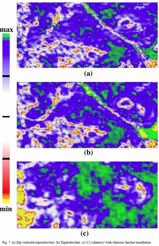
Dip corrected eigenstructure (Figure 7a) provides good strati graphic details as normal C3 eigenstructure coherency (Figure 7b). In places, as in the former example, the dip corrected eigenstructure provides more continuity, as for example, the paleochannel crossing from left upper conner to the lower rigth corner of the figures is clearly depicted, and even more continuous with the dip corrected eigenstructure than for single eigenstructure. In C2 coherency, obtained by using a chinesse checker tessellation, this paleochannel remains hidden (Figure 7c).

4. Conclusions

This study has shown that it is possible to determine apparent dips from a set of seismic traces by means of optimization techniques. We tested the simplex and the Levenberg–Marquardt algorithms. The search of the maximal value from the objective function, the semblance–based coherency, can indeed be optimized by these two numerical techniques. These two optimization techniques were tested with real seismic data. To assess their performance, and for comparative purposes, the direct search strategies (rectangular, polar, and Chinese checker tessellations) were also used with the same data sets. Accordingly, the conclusions are the following:

1.– The direct search strategies provide relative good resolution. Fast estimations from the coherency are obtained in general by means of the polar and Chinese checker tessellations. The rectangular tessellation is a relatively slow technique but with a good resolution. Having the rectangular checker tessellation the best relative performance.

2.– The polar and Chinese checker tessellations for certain range of dp and dq values are quicker that the Simplex technique. Nevertheless, for dp and dq values lower that certain threshold, the Chinese checker tessellation (the fastest of the direct search strategies) requires larger computing times than the simplex technique.

3.– The Levenberg–Marquardt algorithm is the relatively worst one.

4.– The overall comparative analysis shows that among all the techniques, it is the simplex that always provides the highest values under all circumstances for the semblance–based coherency. This result implies that simplex achieves the maximization process more efficiently, while the other analyzed techniques converge towards the solution region but fail attaining the same maxima. This features enables better contrasting between highly and poor coherent zones delimiting the geological features being imaged (e.g., a meandering channel).

5.– Also, small dp and dq values are required to obtain as high coherency values as with the simplex technique, penalizing severely the computing times, but needed to achieve a high resolution mapping of geological features of interest.

6.– Although some of the direct search strategies were fast and displayed good resolution, in our opinion, the simplex technique produces better solutions of coherency values in the shortest time, and thererfore, provides the most reliable apparent dips in comparison with the Levenberg–Marquardt technique and the direct search strategies tessellations.

7.– We achieved to obtain as good resolution with the "deep corrected eigenstructure" as with the C3 coherency (eigenstructure). In our procedure, we first optimize the C2 coherency to estimate the apparent dips; subsequently we slanted the data traces using these dips, and to finally, proceed to calculate the C3 coherency. This "dip corrected C3 eigenstructure", enhances partially the resolution of the conventional C3 coherency. This tells us that volumetric seismic attributes (those calculated in a subvolume of seismic data in a 3–D survey) can enhance their resolution if they follow the orientation of reflectors described by the apparent dips. How to effectively integrate the dips into the estimation of the C3 coherency is an interesting research topic. We currently are focused in such a study.

 

Acknowledgments

We thank very much Dr. Mario Guzmán Vega, head of the Exploration Program at the Instituto Mexicano del Petróleo, and the project D.00397 for making possible these experiments.

 

Bibliography

BAHORICH, M. S. and S. FARMER, 1995. The coherency cube, The Leading Edge, 14(10), 1053–1058.        [ Links ]

BAHORICH., M. S. and S. FARMER, . Techniques of seismic signal processing and exploration.         [ Links ] U. S. Patent No 5, 949, 1996.

BOX, G. E. P. and N. R., DRAPER, 1969. N. R., Evolutionary Operation, John Wiley & Sons, Inc., New York.        [ Links ]

BOX, G. and N. R. DRAPER, 1969. Evolutionary operation: A statistical technique for process improvement, John Wiley and Sons, New York.        [ Links ]

GERSZTENKORN, A. and K. J. MARFURT, 1999. Eigenstructure–based coherence computations as an aid to 3–D structural and strati graphic mapping, Geophysics, 64–5, 1468–1479.        [ Links ]

GOLUB, G. H. and C. F. VAN LOAN, 1983. Matrix computations, John Hopkins Univ. Press.        [ Links ]

LU, WENKAIAND YANDONGLI, SHANWEN ZHANG, HUANQIN XIAO and YANDA LI, 2005. Higher order statistics and supertrace based coherence estimation algorithm. Geophysics, 70, 13–18.        [ Links ]

MARFURT, K. J., R. L. KIRLIN, S. L. FARMER and M. BAHORICH, 1998. 3–D seismic attributes using a semblance–based coherency algorithm. Geophysics, 63, 1150–1165.        [ Links ]

MARFURT, K. J., V. SUDHAKER, A. GEZTERNKORN, K. D. CRAWFORD and S. NISSEN, 1999. Coherency calculations in the presence of structural dip. Geophysics, 64, 104–111.        [ Links ]

MARFURT, K. J. and R L. KIRLIN, 2000. 3–D broad–band estimates of reflector dip and amplitude. Geophysics, 65, 304–320.        [ Links ]

NEIDELL, N. S. and M. T., TANER, 1971. Semblance and other coherency measures of multichannes data. Geophysics, 36, 482–497.        [ Links ]

NELDER, J. A. and R., MEAD, 1965. A Simplex Technique for Function Minimization. Comp. J., 7, 308–313.        [ Links ]

RAO, S. S., 1996. Engineering optimization, John Wiley and sons, New York.        [ Links ]

SPENDLEY, W., G. R. HEXT and F.R. HIMSWORTH, 1962, Sequential Application of Simplex Designs in Optimization and Evolutionary Operation. Technometrics, 4, 441–461.        [ Links ]