


Servicios Personalizados
Revista
Articulo
 Inglés (pdf)
 Artículo en XML
 Referencias del artículo
 Enviar artículo por email
Indicadores
-
 Citado por SciELO
 -
 Accesos
Links relacionados
-
 Similares en
SciELO
Similares en
SciELO
Compartir

 Permalink
Geofísica internacional
versión On-line ISSN 2954-436Xversión impresa ISSN 0016-7169
Geofís. Intl vol.46 no.1 Ciudad de México ene./mar. 2007
Geofísica internacional
Are northeast and western Himalayas earthquake dynamics better "organized" than Central Himalayas: An artificial neural network approach
S. Sri Lakshmi1 and R. K. Tiwari2
1 Theoretical modeling group, National Geophysical Research Institute (NGRI), Uppal Road, Hyderabad – 500 007, INDIA
2 Theoretical modeling group, National Geophysical Research Institute (NGRI), Uppal Road, Hyderabad – 500 007, INDIA. Corresponding Author: Tel.: +91–40–23434648 (Office) Fax: +91–40–27170491/27171564 E–mail: rk_tiwari3@rediffmail.com
Received: July 31, 2006
Accepted: February 14, 2007
Resumen
Los Himalayas entre los 20 y 38 grados de latitud N y los 70 a 98 grados de longitud E están entre las regiones más activas y vulnerables a los temblores en el mundo. Se examina la evolución de la sismicidad en el tiempo (M > 4) en los Himalayas centrales, occidentales y del Noreste para el intervalo de 1960–2003 utilizando el método de redes neuronales artificiales (ANN). El modelo de capas múltiples sirve para simular la frecuencia de sismos con una resolución mensual. Para el entrenamiento del ANN se utiliza un algoritmo de propagación en reversa con optimización de gradiente, y se generaliza el resultado con validación cruzada. Se concluye que las tres regiones se caracterizan por procesos que evolucionan en un plano multidimensional caótico similar a una dinámica auto–organizada. El sector central posee un coeficiente de correlación más bajo que las otras dos regiones, que parecen estar mejor "organizadas", lo que es consistente con la información geológica y tectónica disponible.
Palabras clave: Himalayas, redes neuronales, auto organización, sismicidad.
Abstract
The Himalaya covering 20–38° N latitude and 70–98° E longitude, is one of the most seismo–tectonically active and vulnerable regions of the world. Visual inspection of the temporal earthquake frequency pattern of the Himalayas indicates the nature of the tectonic activity prevailing in this region. However, the quantification of this dynamical pattern is essential for constraining a model and characterizing the nature of earthquake dynamics in this region. We examine the temporal evolution of seismicity (M > 4) of the Central Himalaya (CH), Western Himalaya (WH) and Northeast Himalaya (NEH), for the period of 1960–2003 using artificial neural network (ANN) technique. We use a multilayer feedforward artificial neural network (ANN) model to simulate monthly resolution earthquake frequency time series for all three regions. The ANN is trained using a standard back–propagation algorithm with gradient decent optimization technique and then generalized through cross–validation. The results suggest that earthquake processes in all three regions evolved on a high dimensional chaotic plane akin to "self–organized" dynamical pattern. Earthquake processes of NEH and WH show a higher predictive correlation coefficient (50–55%) compared to the CH (30%), implying that the earthquake dynamics in the NEH and WH are better "organized" than in the CH region. The available tectonogeological observations support the model predictions.
Key words: Himalaya, neural networks, self–organisation, seismicity.
Introduction
The Himalayas are seismo–teectonically one of the most active regions of the world. Visual inspection of changes in the monthly earthquake frequency pattern indicate thath the earthquake dynamics in this region are complex and chaotic in nature possibly due to the prevailing tectonic activities. The available historical data and their appropriate analysis by using the modern powerful signal processing techniques are vital to dissect the nature of earthquake dynamics in these regions.
Some earlier studies of Himalayas and Northeast India (NEI) earthquake data have provided contrasting evidence for the presence of randomness and a low dimensional "strange attractor". Dasgupta et al., (1998) studied the temporal occurrence of earthaquakes for magnitude greater than or equal to 5.5 and 6.0 (for two different data sets) for NEI using the Poisson probability density function analyses. The analysis indicates that the temporal pattern in this region follow Poisson distribution. Srivastava et al. (1996) applied the G–P algorithm (Grassberger and Procaccia, 1983) to the NEI earthquake time series and suggested that the earthquake dynamics in this region are governed by low dimensional chaos.
In the present paper, we have applied the artificial neural network (ANN) technique for the Himalayan major tectonics units, Northeast Himalayas (NEH), western Himalayas (WH) and central Himalayas (CH). Artificial neural network (ANN) is a powerful method, which is being invariably used for modeling different types of data. The major advantage of ANN is its ability to represent the underlying nonlinear dynamics of a system modeled without any prior assumption information and regarding the processes involved. In the geophysical domain, neural networks have been applied in various fi elds (Chakraborthy et al., 1992; Tao & Du, 1992; Feng et al., 1997; Arora and Sharma, 1998; Bodri, 2001; Manoj and Nagarajan, 2003). The application and comparisons of theses results with earlier results of nonlinear analysis will reduce bias and also provide better confi dence for understanding the underlying physical processes that are responsible for the dynamical nature.
Tectonics and Seismicity of Himalayas
Tectonic Features of Himalayas
The tectonics and seismicity of the Himalayas have been studied and discussed by many researchers during the past few years (Molnar et al., 1973; Seeber et al., 1981; Ni and Barazangi, 1984; Molnar, 1990). The main tectonic features of the Himalaya and the adjoining regions are shown in Figure 1 (Gansser, 1964). The major faults from north to south in the Himalayas are: the Trans–Himalayan Fault (THF), the Main Central thrust (MCT), the Main Boundary Thrust (MBT) and the Himalayan Frontal Fault (Gansser 1964; Kayal, 2001).
Most of the earthquake events occurring in this region are concentrated along the thrust zones. The occurrence of earthquakes is confi ned to crustal depths of about 20 kms (Ni and Barazangi, 1984). Global Positioning System (GPS) measurements show that India and Southern Tibet converge at 20 ± 3 mm/yr (Larson et al., 1999). Evidence also shows localized vertical movement in this region (Jackson sand Bilham, 1994) and small earthquakes are most common (Pandey et al., 1995).
The seismicity associated in this region is mainly underthrusting of plates (Molnar et al., 1973; Ni and Barazangi, 1984). The sections of the plate boundary that have not been ruptured during the past 100 years are called as the seismic gaps and are estimated to be the main candidate locations of the occurrence of future great earthquakes. The section west of the 1905 Kangra earthquake is referred as the Kashmir gap; the section between the 1905 Kangra earthquake and the 1934 Bihar earthquakes is the Central gap; the section between the 1934 and 1950 Assam earthquakes is referred as the Assam gap. The westernmost gap is mainly called location of complex earthquakes (Khattri et al., 1983; Khattri, 1987).
Great Earthquakes in the Himalayas
Many major earthquakes of differing size that have occurred during the past centuries dominate the seismicity of the Himalayan region. The major ones among them are: 1897 earthquake associated with the rupture in the south of Himalaya beneath the Shillong plateau (and the formation of the Shillong plateau, M=8.7); the 1905 Kangra earthquake (M=8.6); the 1934 Bihar–Nepal earthquake (M=8.4) and the 1950 Assam earthquake (M=8.7) (Richter, 1958). In addition to these, a few more earthquakes of magnitude M > 7 have occurred during the years 1916 (M=7.5), 1936 (M=7.0) and 1947 (Molnar, 1990). During the last decade, three significant and damaging earthquakes with M > 6.5 have occurred in Himalayas in 1988 (M=6.6), 1991 (M=6.6) , 1991 (M=6.6) and 1999 (M=6.3) (Kayal, 2001; Tiwari, 2000).
The whole of Himalayas covering 20–38° N and 70–98° E (Teotia et al., 1997) is divided approximately into three zones: (i) Central Himalayas (28–38° N latitude and 78–98° E longitude) (ii) Northeast Himalayas (20–28° N latitude and 88–98° E longitude) (Gupta et al., 1986) and (iii) Western Himalayas (30–38° N latitude and 70–78° E longitude). The data used here are mainly from the NOAA and USGS earthquake catalogues complied for the period of 1960 to 2003 for magnitude M > 4 events. The monthly frequency data has been prepared for these three regions i.e. the number of events per month has been prepared from 1960 to 2003 (i. e. 44 years X 12 (as 1 year = 12 months) = 528 months or events. Figure 2 shows the spatial distribution of the earthquake events in the Himalayas in the three zones CH, NEH and WH respectively.
Characterization of dynamical nature of the Himalayan earthquake time series
Artificial neural networks (ANN)
The techniques of artificial neural networks (ANN) are promising solutions to various complex problems that work on the principle of structure of brains and nerve systems (Poulton, 2002). Among the different algorithms, the Back–propagation is most commonly used (Werbos, 1974; Rumelhart and McClelland, 1986; Lippmann, 1987) and has been applied successfully to a broad range of fi elds such as speech recognition, pattern recognition, and image classification.
Appropriate Architecture design of ANN for the present problem:
An ANN usually has an input layer, one or more intermediate or hidden layers and one output layer which produces the output response of the network. When a network is cycled, the activations of the input units are propagated forward to the output layer through the connecting weights. Inputs could be connected to many nodes with various weights, resulting in a series of outputs, one per node. The connections correspond roughly to the axons and synapses in a biological system, and they provide a signal transmission pathway between the nodes. The layer that receives the inputs is called the input layer. It typically performs no function other than the buffering of the input signal. The network outputs are generated from the output layer. Any other layers are called hidden layers because they are internal to the network and have no direct contact with the external environment. There may be zero, to several hidden layers. The connections are multiplied by the weights associated with that particular interconnect. The architecture of the multilayered ANN neural network is shown in Figure 3.
Backpropagation Algorithm:
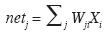
The network used in this paper is the most popularly used back propagation–learning algorithm or the Generalized Delta Rule (Pao, 1989). Like the perceptron, the net input to a unit is determined by the weighted sum of its inputs
 ..................................................................(1)
where Xi is the input activation from unit i and Wji is the weight connecting unit i to unit j. However, instead of calculating a binary output, the net input is added to the unit's bias θ and the resulting value is passed through a sigmoid function
 .....................................................(2)
Learning in a backpropagation network occurs in two steps: First each pattern Ip is presented to the network and propagated forward to the output. Second, a method called gradient descent is used to minimize the total error on the patterns in the training set. In gradient descent, weights are changed in proportion to the negative of an error derivative with respect to each weight
 .........................................................(3)
Weights move in the direction of steepest descent on the error surface defi ned by the total error (summed across patterns) i. e.
 .....................................................(4)
where opj be the activation of output unit uj in response to pattern p and tpj is the target output value for unit uj. After the error on each pattern is computed, each weight is adjusted in proportion to the calculated error gradient backpropagated from the outputs to the inputs. The changes in the weights reduce the overall error in the network.
Selection of parameters used for training:
Here the earthquake monthly frequency data has been taken as the input values for the neural network modeling. The data is split into three sets i.e., one–fourth for the validation set, one fourth for the test set and the remaining one half for the training set. There is no unique criterion or method that provides rules for the optimal division of the underlying data sets. The occurrence of the earthquake of a given year or month is dependent on the previous years or months (1, 2, 3, 4,.......). Here time–delay neural network input is used, i.e., the input data to the network is selected as a temporal sequence of the previous monthly frequency data. The output is the frequency value for the next month.
The notation i–j–k will be used to label an ANN with input (i), hidden (j), and output (k) neurons. The input layer is chosen to contain 5 neurons and one output neuron representing the modeling result. The number of hidden–layer neurons was altered to optimize the results achievable with this type of network by changing them in between 2 and 20 neurons. Hence fi nally 10 hidden nodes are selected for the training process. The optimal neural network topology was obtained and denoted as 5–10–1: A sigmoid transfer function was used for the hidden layer, and a linear function was used for the output layer. All weights were initialized to random values between –0.1 and 0.1. The learning rate and momentum relate the variation of the weights to the gradient of the error function. They were set to 0.5 before training and then optimized on a trial basis during the training procedure. Thus the learning rate and momentum are 0.01 and 0.9 respectively.
Training the network:
The performance of the ANN was tested on a testing data set (a subset of the data set) and monitored during the learning procedure to determine when the learning process had to be stopped. An early stopping strategy was adopted in this work to avoid overtraining i.e., when the descending rate of training error was small enough and the testing error began to increase, the learning procedure stopped. The data is presented and error is calculated for each input then it is summed and compared with desired error. If it does not match with the desired error, it is fed back (back propagated) to the neural network by modifying the weights, until the error decreases with each iteration and the neural model gets closer and closer to producing the desired output. This process is known as "training" or "learning".
The training data set is used to select and identify an optimal set of connection weights, the testing set for choosing the best network confi guration. Once the optimal network has been identifi ed, the validation set is required to test the true generalization ability of the model. The validation data should not be used in training but instead is reticent for the quality check of the obtained work. Training is stopped when there is unsatisfactory misfi t between the training set and the testing set. There are two phases in the training cycle, one to propagate the input pattern and the other to adapt the output. It is the errors that are backward propagated in the network iteration to the hidden layer (s). During the neural network training each hidden and output neurons process the inputs by multiplying them with their weights. The products are thereby summed and processed using an activation function like sigmoid, tan sigmoid etc. The network is trained by using the generalized Delta Rule. This method is used to fi nd a suitable solution for a global minimum in the mismatch between the desired and the actual value. The degree of error is calculated and then the error is propagated backwards through the network by adjusting the parameters between the hidden and the input layer, i. e. the errors are backward propagated in the network iteration to the hidden layer (Rumelhart and McClelland, 1986).
Model Characterization and evaluation of model performance
Test on some simple theoretical models:
The predictability of a system or time series is related to the number of degrees of freedom in generating the dynamics. This can be studied clearly with reference to the results of some non–linear models like stochastic, chaotic or logistic and random models. The concept of determinism plays a central role in the evolution of physics, which suggests the possibility of predicting a future evolution on the basis of its initial conditions.
Stochastic model: The stochastic models are generally used to describe all the systems that are governed by a large number of degrees of freedom. The autoregressive (AR) model is one of examples of such a processes. A fi rst order autoregressive (AR) model or random walk model (Fuller, 1976) can be given in the form
 .....................................................................(5)
where i = 1,2,3,4.........N, denotes the discrete time increment,  is lag–one autocorrelation coefficient and describes the degree of signal correlation in the noise and is calculated from the data which has value
  0.5, and βi is (stationary) purely random process (normal independent random variables uniformly distributed in the interval (0,1)). Xi depends partly on Xi–1 and partly on the random disturbance βi.
Chaotic model: A "logistic model" (May, 1976) represents the chaotic dynamics. The mathematical form of the logistic model can be given as:
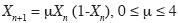 ....................................................(6)
where Xn, control parameter is the relative values ranging from 0 to 1, and µ, is the coefficient (the control parameter) between 0 and 4 (May, 1976).
Random model: Random noise is uncorrelated, has zero mean, and is not predictable due its uncorrelated nature. Time series of random numbers have oscillations ranging from different amplitudes and thus produce a fl at continuum.
Application of ANN on mathematical models and their comparison:
The efficiency of the ANN network is fi rst tested on the theoretical models (chaotic, stochastic and random models) and then to the original time series. After the training has been completed, the correlation coefficients between the observed (original time series) and predicted values were calculated for the three models e.g. chaotic, stochastic and random. Figure 4 shows plots of predicted values against observed values for chaotic, stochastic and random processes, respectively. From the Figure 4, it is visible that among the three models, the chaotic model shows better predictability for limited data than the stochastic model and the random model. In fact random model shows random scatter with zero correlation. The stochastic model predicts only 45% of the data. This is obviously an inherent quality of these models. The value of the correlation coefficient between the observed and predicted values for the three models using ANN approach is shown in Table 2.
Comparison of the correlation coefficient values for the three tectonic zones of the Himalayas
The earthquake monthly frequency data sets of the three tectonic units of the Himalayas i.e. WH, NEH and CH were trained using 5 input neurons. The best–fi tted network models are calculated. Examining errors on the training, validation and testing data sets can test the performance of a trained network, but it is often useful to investigate the network response in much more detail. One option to do so is to perform a regression analysis between the network response and the corresponding targets. The comparison between the observed and predicted values for the three tectonic units is shown in Figure 5. The results are plotted with the actual (observed) values on the X–axis and the predicted (calculated) values on the Y–axis for all the three tectonic zones. The network outputs are plotted versus the targets as dots. A dashed line indicates the best linear fi t. The solid line indicates perfect fi t (output equal to targets). If a perfect fi t is observed (outputs exactly equal to targets), the slope would be 1, and the y–intercept would be zero. The correlation coefficient (R–value) between the outputs and targets is a measure of how well the variation in the output is explained by the targets. If this number is equal to 1, then there is perfect correlation between targets and outputs. For all the earthquake data, we fi nd the value of correlation coefficient between the observed and predicted values by using the ANN approach for the three zones to range from is 0.3 to 0.52 (Table 3).
Correlation coefficient values for NEH (R=0.519) and WH (R=0.538) are almost the same suggesting that the earthquake generating processes in these regions is almost similar. In order to quantify the differences between the actual and predicted values, the sum–squared errors are calculated for all the three tectonic units. The sum–squared error here is the sum of the squared differences between the network targets and the actual outputs for a given set of values. It is a diagnostic tool to plot the training, validation and testing errors to check the progress of training. Figure 6 shows the sum–squared error for the WH, CH and NEH respectively. The sum–squared error should reach constant values when the network converges. From the Figure 6 it is observed that the training stopped after 15 to 20 iterations for all the three tectonic regions because the validation error increased. The result obtained is valid and reasonable as the test set errors and the validation set errors have similar characteristics, and do not shown any significant overfi tting in the plot. Thus the ANN model obtained provides a reasonably good fi t between the observed and predicted values indicating the feasibility of the ANN method for such analyses.
Discussions and conclusions
In this paper, the modern technique of artificial neural networks (ANN) is employed to study the dynamical behavior of the earthquake time series of the Himalayas and its contiguous regions. It is a good strategy to make use of distinct diagnostic methods to characterize complexities in observational time series. The above technique has been applied to the monthly frequency earthquake time series data in an attempt to assess the predictive behavior of earthquake occurrences in these regions (WH, CH and NEH) and thereby characterizing the nature of the system's dynamics (e.g. random/stochastic/chaotic). Present analyses of monthly earthquake frequency time series using ANN emphasize the presence of high dimensional chaos in the entire tectonic units of Himalayas e.g. NEH, WH and CH because the correlation coefficients calculated between predicted and actual earthquake frequency values are in the range of 30 to 55% in almost all the cases. Obviously, if the correlation coefficients (McCloskey, 1993) are significantly greater than 50%, one may consider the underlying processes to obey low dimensional chaotic dynamics, otherwise high dimensional chaos. The present results rather suggest that earthquake–generating mechanism in these regions are dominated by stochastic and/or high dimensional chaos. These results correlate well with the results obtained by the nonlinear forecasting (Tiwari et al., 2003; Tiwari and Srilakshmi, 2005). (see also Tables 2 and 3)
Both the methods exhibit almost the same range of values of predictive correlation coefficient ranging between 0.3–0.55, indicating that both the methods reveal the presence of high dimensional chaos in this region (Tiwari et al., 2003, 2004; Tiwari and Sri Lakshmi, 2005). The slight deviations in the correlation coefficient values obtained by the ANN might be due to the better training performance of the network. Note that, despite the different approaches of analysis, the predictive correlation coefficient is almost similar suggesting that the result is stable.
Another interesting observation of the present study, which is also geo–tectonically important, is that the present ANN technique shows better determinism for NEH and WH earthquake data (high correlation coefficient) as compared to CH. The reason for this finding can be a geological one as it may be closely linked to the underlying seismo–tectonic processes invoking the dynamics of the system. The three tectonic regions display distinct tectonic activities and features: NEH and WH appear to high strain rate) characteristics that have been affected by Cretaceous magmatism plume activity (Tiwari and Srilakshmi, 2005). In contrast, the CH due to under thrusting of the Bundelkhand craton is likely to be a region of comparatively low stress rates. The strain rates in NEH and WH are almost 1–2 times larger than the strain rates in CH. It may also be significant that the CH arc (a region intersecting between the eastern Himalayan arc and western Himalayan arc i.e around 80°–86°E) has remained comparatively quiescent or there have been less earthquake activities. Hence, the relative seismic quiescence of the central Himalayas has widely been termed as seismic gap (Khattri et al., 1983, Khattri, 1987) implying that, even though, the stress is continuously building up falling the ongoing convergence between India and Eurasia it is not getting released in this zones.
These results may have important implications for the study of dynamical behavior of earthquake generating mechanism in the Himalayas. The Himalayan time series of earthquakes of size with magnitude 4 and higher is modeled by high number of variables i.e., better modeled by the stochastic or a high–dimensional process. The application of the (ANN) is helpful for the study of nonlinear dynamical system in the earthquake time series.
We can summarize our results as follows:
(1) The available earthquake data in the WH, CH and NEH show evidence for high dimensional deterministic chaos suggesting that the earthquake dynamics in these regions are highly unpredictable. It is therefore somewhat difficult, at this stage, to conclude specific reasons responsible for the complex occurrences of earthquake dynamics in these regions.
(2) ANN analysis suggests that the earthquake dynamics in NEH and WH are better organized than in CH region.
(3) The study might provide useful insight for constraining the models of crustal dynamics (using available multi–parametric geophysical and geological data for Himalayan earthquakes in this region) and seismic hazard study.
Acknowledgements
One of the authors, Dr. S. Sri Lakshmi expresses her sincere thanks to CSIR for providing the Research Associate Fellowship (RA) to carry out the research work. We are thankful to Dr. V. P. Dimri, Director of the National Geophysical Research Institute, Hyderabad for his kind permission to publish the manuscript.
Bibliography
ARORA, M. and M. L. SHARMA, 1998. Seismic hazard analysis: An artificial neural network approach. Current Science 75, 1, 54–59. [ Links ]
BODRI, B., 2001. A neural–network model for earthquake occurrence,.J. Geodynamics 32, 289–310. [ Links ]
CHAKRABOTRY, K., K. MEHROTRA, C. MOHAN and S. RANA, 1992. Forecasting the behavior of multivariate time series using neural networks. Neural Networks 5, 961–970. [ Links ]
DASGUPTA, S., A. BHATTACHARYA and K. JANA, 1998. Quantitative assessment of seismic hazard in Eastern–Northeastern. J. Geol. Soc. of India 52, 181–194. [ Links ]
FENG, X., M. SETO and K. KATSUYAMA, 1997. Neural dynamic modeling on earthquake magnitude series, Geophys. J. Inter., 128, 547–556. [ Links ]
FULLER, W. A., 1976. Introduction to statistical time series, John Wiley and Sons, New York. [ Links ]
GANSSER, A., 1964. The Geology of the Himalayas, Wiley–Interscience, New York, 298 pp. [ Links ]
GRASSBERGER, P. and I. PROCACCIA, 1983. Measuring the strangeness of strange attractors: Physica 9D, 189–208. [ Links ]
GUPTA, H. K., K. RAJENDRAN and H. N. SINGH, 1986. Seismicity of the northeast Indian region. J. Geol. Soc. India 28, 345–365. [ Links ]
JACKSON, M. and R. BILHAM, 1994. Constraints of Himalayan deformation inferred from vertical velocity fi elds in Nepal and Tibet. J. Geophys. Res. 99, 13897. [ Links ]
KAYAL, J. R., 2001. Microearthquake activity in some parts of the Himalaya and the tectonic model. Tectonophysics 339, 331–351. [ Links ]
KHATTRI, K .N., 1987. Great earthquakes, seismicity gaps and potential for earthquake disaster along the Himalayan plate boundary. In: K. Mogi and K.N. Khattri (Eds.), Earthquake Prediction. Tectonophysics 138, 79–92. [ Links ]
KHATTRI, K., M. WYSS, V. K. GAUR, S. H. SAHA and V. K. BANSAL, 1983. Local seismic activity is the region of the Assam gap, northeast India. Bull. Seism. Soc. Am., 73, 459–469. [ Links ]
LARSON, K., R. BURGMANN, J. BILHAM and J. FREYMUELLER, 1999. Kinematics of India–Eurasia collision zone from G.P.S measurements. J. Geophys. Res, 104, 1077. [ Links ]
LIPPMANN, R. P., 1987, An Introduction to computing with neural networks. IEEE ASSP Magazine 4, 2, 4–22. [ Links ]
MANOJ, C. and N. NAGARAJAN, 2003, The application of artificial neural networks to magnetotelluric time–series analysis. Geophys. J. Int., 153, 409–423. [ Links ]
MAY, R., 1976. Simple mathematical models with very complicated dynamics. Nature 261, pp. 459–467. [ Links ]
McCLOSKEY, J., 1993. A hierarchical model for earthquake generation on coupled segments of a transform fault, Geophys. J. Inter., 115, 538–551. [ Links ]
MOLNAR, P., 1990. A review of the seismicity and the rates of active underthrusting and deformation at the Himalaya. Jour. of Himalayan geology 1(2), 131–154. [ Links ]
MOLNAR, P., T. J. FITCH and F. T. WU, 1973. Fault plane solutions of shallow earthquakes and contemporary tectonics in Asia. Earth and Planet. Sci. Lett. 19, 101–112. [ Links ]
NI, J., and M. BARAZANGI, 1984. Seismotectonics of the Himalayan collision zone: geometry of the underthrusting Indian Plate beneath the Himalaya. J. Geophys. Res., 89, 1147–1163. [ Links ]
PANDEY, M., R. P. TANDUKAR, J. P. AVOVAC, J. LAVE and J. P. MASSOT, 1995, Interseismic strain accumulation on the Himalayan Crustal Ramp (Nepal), Geophys. Res. Lett., 22, 751. [ Links ]
PAO, Y. H., 1989. Adaptive Pattern recognition and Neural network, Addison–Wesley, reading, Mass. [ Links ]
POULTON, M., Ed., 2002. Neural networks as an intelligence amplification tool: A review of applications. Geophysics 67, 3, 979–993. [ Links ]
RICHTER, C. F., 1958. Elementary Seismology, W. H. Freeman, San Francisco, 47–65, 709–715. [ Links ]
RUMELHART, D. E., G. E. HINTON and R. J. WILLIAMS, 1986. Learning internal representation by back propagating errors. Nature 332, 533–536. [ Links ]
RUMELHART, D. E. and J. L. McCLELLAND, 1986. Parallel Distributed Processing, MIT Press, Cambridge, Massachusetts, 318–362. [ Links ]
SEEBER, L., J. G. ARMBRUSTER and R. QUITTMEYER, 1981. Seismicity and continental subduction in the Himalayan arc. In: H. K. Gupta and F. M. Delany (Editors), Hindu Kush, Himalaya: Geodynamic Evolution, Geodynamic Series, Am. Geophys. Union 3, 215–242. [ Links ]
SRIVASTAVA, H.N., S. N. BHATTACHARYA and K. SINHA ROY, 1996. Strange attractor characteristics of earthquakes in Shillong plateau and adjoining region, Geophys. Res. Lett. 23, 24, 3519–3522. [ Links ]
TAO, X.X. and W. DU, 1992. Seismicity trends along the southeastern coastal seismic zone assessed by artificial neural networks. Earthquake Res. in China, 6, 91–98. [ Links ]
TEOTIA, S. S, K. N. KHATTRI and P. K. ROY., 1997. Multifractal analysis of seismicity of the Himalayan region. Current Science 73, 4, 359–366. [ Links ]
TIWARI, R. K. and S. SRILAKSHMI, 2005. Some common and contrasting features of earthquake dynamics in the major tectonic units of Himalayas using the non–linear forecasting approach. Current Science 88, 640–647. [ Links ]
TIWARI, R. K., S. SRILAKSHMI and K. N. N. RAO, 2003. Nature of earthquake dynamics in the central Himalayan region: a nonlinear forecasting analysis. J. Geodynamics 35, 273–287. [ Links ]
TIWARI, R. K., S. SRILAKSHMI and K. N. N. RAO, 2004. Characterization of earthquake dynamics in Northeastern India regions: A modern nonlinear forecasting approach, PAGEOPH 161, 4, 865–880. [ Links ]
TIWARI, R. P., 2002. Status of seismicity in the northeast India and earthquake disaster mitigation. ENVIS Bulletin 10, 1, 11–21. [ Links ]
WERBOS, P. J., 1974. Beyond regression: new tools for prediction and analysis in the behavioral sciences: unpublished Masters thesis, Harvard University, Cambridge, Massachusetts, 453 pp. [ Links ]

