


Servicios Personalizados
Revista

Articulo
 Inglés (pdf)
 Artículo en XML
 Referencias del artículo
 Enviar artículo por email
Indicadores
 Citado por SciELO
 Links relacionados
-
 Similares en
SciELO
Similares en
SciELO
Compartir

 Permalink
Geofísica internacional
versión On-line ISSN 2954-436Xversión impresa ISSN 0016-7169
Geofís. Intl vol.45 no.3 Ciudad de México jul./sep. 2006
Estimation of hydraulic conductivity on clay content in soil determined from resistivity data
Vladimir Shevnin1, Omar Delgado–Rodríguez1, Aleksandr Mousatov1 and Albert Ryjov2
1 Mexican Petroleum Institute, Eje Central Lázaro Cárdenas 152, 07730, Mexico D.F. E–mail: vshevnin@imp.mx
2 Moscow State Geological Prospecting Academy, Geophysical faculty, Volgina str., 9, 117485, Moscow, Russia.
Received: May 6, 2005
Accepted: August 1, 2006
Resumen
El contenido de arcilla en suelos areno–arcillosos influye sobre la permeabilidad hidráulica (coeficiente de filtración). Se presenta una revisión de datos experimentales publicados que relacionan el coeficiente de filtración con el tipo litológico del suelo y el tamaño de las partículas. A partir de cálculos teóricos, se modifican las conocidas fórmulas que relacionan el coeficiente de filtración con el contenido de arcilla. Se estima el contenido de arcilla a partir de los datos interpretados por el método SEV, y se propone un procedimiento para la estimación del coeficiente de filtración: (a) cálculo del contenido de arcilla a partir de la resistividad del suelo y de la salinidad del agua subterránea, (b) estimación del coeficiente de filtración a partir del contenido de arcilla. Se presentan algunos ejemplos de la aplicación de esta metodología.
Palabras clave:: Permeabilidad hidráulica, contenido de arcilla, suelos areno–arcillosos, Sondeo Eléctrico Vertical, Imagen de Resistividad 2D, modelación petrofísica.
Abstract
The influence of clay content in sandy and clayey soils on hydraulic conductivity (filtration coefficient) is considered. A review of published experimental data on the relationship of hydraulic conductivity with soil lithology and grain size, as dependent on clay content is presented. Theoretical calculations include clay content. Experimental and calculated data agree, and several approximation formulas for filtration coefficient vs clay content are presented. Clay content in soil is estimated from electric resistivity data obtained from 2D VES interpretation. A two–step method is proposed, the first step including clay content calculating from soil resistivity and groundwater salinity, and the second step including filtration coefficient estimating from clay content. Two applications are presented.
Key words: Hydraulic conductivity, clay content, sandy clayey soils, Vertical Electrical Sounding, 2D Resistivity Imaging, petrophysical modeling.
Introduction
Hydraulic conductivity is an important parameter in hydrogeology. This parameter is useful for groundwater management, groundwater protection and prediction of contaminants transport.
Standard techniques to determine hydraulic conductivity, such as pump tests, tracer tests or grain size analysis, require boreholes, which turn out to be relatively expensive, with sparse results and low resolution of the resulting maps. Superficial geophysical methods, such as resistivity or vertical electrical sounding (VES) require no perforation, and can produce information faster and with higher resolution. But soil resistivity has no direct theoretical relationship with the filtration coefficient Kf, which depends on many parameters, such as soil porosity, grain size, capillary radius and clay content. It was found in experiments that Kf decreases as clay content increases, and so does soil resistivity. Thus, we may expect a proportional relationship between soil resistivity and Kf. Soil resistivity depends on other parameters, like groundwater salinity, soil humidity, temperature, etc. For a successful correlation with Kf we need to know these additional parameters or to fix them.
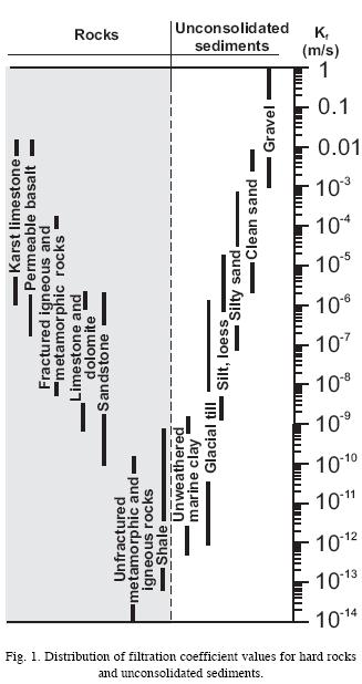
In Figure 1 the intervals of filtration coefficient values for different rocks and unconsolidated sediments are presented. Hydraulic conductivity in rocks exists due to fractures, and in unconsolidated sediments due to intergranular pores. The lowest filtration coefficients for sediments correspond to unweathered marine clay and the highest to clean sand and gravel. We conclude that filtration coefficients for unconsolidated sediments are distributed accordingly to grain size or clay content.
In this work, we consider only loose sandy–clayey soils (unconsolidated sediments). There are different schemes of hydraulic conductivity estimation for sand–clay soils on geoelectrical parameters, correlating hydraulic conductivity with electric resistivity. This correlation is directly proportional on a regional scale (higher resistivity corresponds to higher hydraulic conductivity), but sometimes on a local scale the correlation is inversely proportional (Mazac et al., 1990). When increasing gravel content in sand–clay soil causes an increase in soil resistivity, it will also result in soil porosity and hydraulic conductivity decreasing, and correlation with resistivity can be inversely proportional. In Mazac et al. (1990) the influence of groundwater salinity and clay content on soil resistivity is not taken into account. But clay content evidently influences hydraulic conductivity. When the clay content in soil is rather high (30–100%) and salinity is increasing, hydraulic conductivity and soil resistivity won't change. When in the same area there are sandy lenses, their resistivity diminishes with salinity increase without change of hydraulic conductivity, but sandy lenses have higher hydraulic conductivity in comparison with clayey soil. Such effects can distort the correlation between soil resistivity and hydraulic conductivity.
In several publications (Melkanovitsky, 1984, Geophysical methods ..., 1985) the idea to use transversal resistance (T=ρ*h, where h is the thickness of the subject layer) for hydraulic conductivity estimating was discussed. Parameter T can be found with higher accuracy than resistivity from VES interpretation, because the equivalence principle does not influence T values in the intermediate resistive layer. In this scheme, the influence of groundwater salinity and clay content is not taken into account.
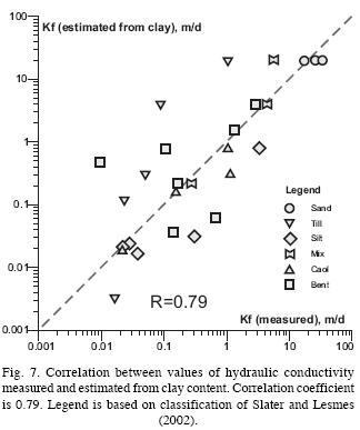
Salem (2001) published a formula relating hydraulic conductivity with formation factor F that allows finding hydraulic conductivity from resistivity data obtained through VES method:
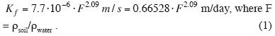
This formula takes into account groundwater salinity (by using F), but it does not consider clay content.
Berg (1970) showed, that in a heterogeneous mixture of different grains, hydraulic conductivity is controlled by the component with the finest pore system, in other words, by clay content.
Clay content influence on filtration coefficient was mentioned in Marion (1990) and Knoll et al. (1995) as an important factor in the relationship between geophysical parameters and hydraulic conductivity for unconsolidated sediments.
Ogilvi (1990) showed the results of filtration coefficient studies in Figure 2.
He obtained the dependency between electric resistivity and filtration coefficient for different conditions of soil humidity and groundwater salinity. This figure and the table below show relationship between soil lithology (sand, sandy loam, loam, clay, with subdivisions for each lithological group), grain size (14 gradations), and filtration coefficient (in bold black frame). Using soil lithology and grain size in this table, we estimated clay content as in bottom row of the table. Between these two rows we created correlation formula (9).
Empirical and theoretical relationships between Spectral Induced Polarization (SIP) and hydraulic conductivity were studied in theory and in the laboratory by Börner et al. (1996) and Slater and Lesmes (2002). Other researchers (Hördt et al., 2005) performed field measurements with SIP method for hydraulic conductivity estimation. But the SIP method is rather complex for fieldwork and needs measurements in broad frequency intervals (at least 4 frequency orders). Therefore, this method is used more in the laboratory than in the field.
According to Börner et al. (1996) hydraulic conductivity can be calculated with the help of the Kozeny – Carman equation on formation factor F and the specific inner surface area S por (estimated from the imaging part of complex conductivity measured with the SIP method):
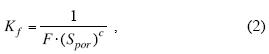
where Kf is filtration coefficient in m/s and Spor= is in 1/μm, Spor = 8.6 . Im(σ), σ is electrical conductivity in S/m, and coefficient c is a constant in the interval 2.8 – 4.6.
According to Slater and Lesmes (2002), Spor related to the imaginary part of superficial conductivity Im(σ ) depends on the specific inner surface area and on Cation Exchange Capacity – CEC (of clay component) and depends little on electrolytic conductivity (of pore water). Slater and Lesmes demonstrated that Im(σ) has correlation with d10 (granulometric parameter) characterizing the fine part of soil component.
At the SAGEEP conference (Shevnin et al., 2006) we demonstrated the possibility to separate, by a petrophysical interpretation of VES data, values of superficial conductivity and electrolytic conductivity. SIP as well as VES allow estimating superficial conductivity in soil pores and finding the filtration coefficient, because superficial conductivity is created mainly by clay or quasi–clay content in soil.
With the help of superficial electrical methods like VES a great volume of non destructive, fast and low–cost electrical measurements is feasible, performing, unlike direct measurements of hydraulic conductivity.
Based on the similarity between electric and water current distribution in clay–sand soils (using the same pore system) it is possible to establish and use a correlation between hydraulic and electric conductivity. The main idea of our study is not to substitute direct hydraulic conductivity measurements for indirect ones, but to integrate them to perform fast and fairly exact estimations of hydraulic conductivity with low cost and high resolution using direct Kf measurements to calibrate indirect geophysical results of Kf estimations.
CALCULATIONS
According to Kozeny theory (Gavich et al., 1983), a porous medium is considered as an ensemble of fine tubes with the same length. Hydraulic conductivity is equal to

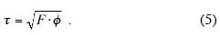
where: Φ is porosity for Kozeny model; d is a tube diameter in mm;  is a tortuosity; A is a constant depending on the units: A=0.92*108 for d in mm and Kf in m/d. Kozeny formula can be applied to sand–clay soil. Hydraulic conductivity is a function of soil porosity, capillary radii and tortuosity. These three parameters are not completely independent; for example, we can calculate tortuosity with the help of formula (5) using soil porosity Φ and formation factor F (Bassiouni, 1994):
For sand –clay soil it is more common to use sand and clay grain size instead of capillary radii. Pore diameter is about 0.1–0.3 of grain diameter. For spherical grains of the same diameter, porosity doesn' t depend on grain diameter, but on grain packing. Sand porosity is equal to 47.64% for cubic packing and 25.95% for hexagonal packing.
In the case of a sand–clay mixture, smaller particles of clay fill the pore spaces between sand grains until clay content remains lower or equal to sand porosity. At higher clay content sand grains become suspended in the clay matrix. Porosity of the mixture can be calculated using sand and clay porosities and clay content (Ryjov and Sudoplatov, 1990; Marion, 1990).
The total porosity Φ of the sandy clay soil is calculated from the following expressions (Ryjov and Sudoplatov, 1990):
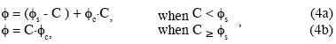
where C is clay content,Φc is clay porosity and Φs is sand porosity. Clay and sand porosities are considered as constant; therefore, soil porosity is a function of clay content.
Thus, porosity, grain size (or capillary radius) and tortuosity are not independent parameters. Rather, they are interrelated in the sand–clay soil model. In this work we use clay content as the main factor, as a function of other parameters such as soil porosity, tortuosity and formation factor.
There are formulas of Kf calculations based on grain diameter (Kobranova, 1986; Salem, 2000).
The formulas of Kf for spheres of the same diameter (Kobranova, 1986) depend on grain packing. For example, for hexagonal packing the expression is:
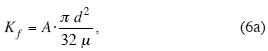
and for cubic packing it is:
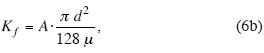
where: d is diameter of sphere in mm; μ is viscosity of fluid; A=0.75*106 (when d is in mm and Kf in m/d). In these formulas, the only factor is grain diameter, but in reality, the porosity influence is hidden in the coefficients, depending on grain packing.
Both capillary radius and porosity are taken into account in the formula (Mironenko and Shestakov, 1978):

where θ is a porosity, R capillary radius; g water density; x tortuosity; A is a constant, depending on units.
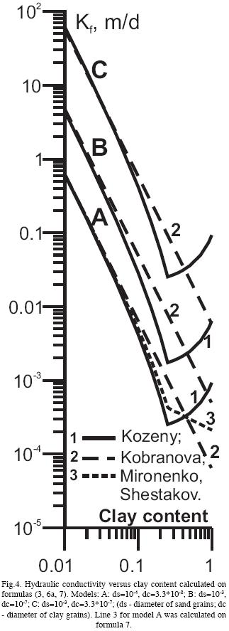
Comparing formulas (6), (7) and (3) we conclude that in formula (6) Kf is proportional to d2, in formula (7) it is proportional to R2. θ. and in formula (3) Kf is proportional to d 2. θ2 / F. The common main factor in all formulas is d2 (or r2). Influence of porosity θ and formation factor F is more noticeable at high clay content. For soil model A in Figure 4 we compared formulas (6), (7) and (3). They give similar results at low clay content and differ at high clay content. Porosity 8 is a minimum where clay content is equal to sand porosity. At the same point the formation factor F has maximum. Thus using formula (3), which contains d 2. θ2 / F, we notice a minimum in the Kf curve.
Expressions (6a, b) do not consider clay content directly. Clay content is present indirectly in d values, in soil grain size, but may be expressed directly taking into account clay content and using the formula (Konishi and Kobayashi, 2005):
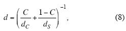
where C is clay content, dc is clay grains diameter, ds is sand grains diameter, and d is the mean value of grain diameters in the soil mixture, with variable clay content.
We calculated Kf using formula (6a), taking into account clay content and using d value with the help of formula (8).
Theoretical graphs of resistivity versus salinity for different clay content values are displayed in Figure (3 A), calculated with Ryjov's algorithm Petrowin (Ryjov and Sudoplatov, 1990; Shevnin et al., 2005). This algorithm also calculates soil porosity as function of clay content in sand–clay soil, using formulas (4a) and (4b) (Figure 3 B). Figure (3 A) can be used to determine clay content from soil resistivity and groundwater salinity. Suppose salinity is 0.01 g/l. If soil resistivity is 2.3 Ohm.m, clay content in this soil according to Figure (3A) is 100%. When resistivity is 10 Ohm.m, clay content is 26%. When soil resistivity is 100 Ohm.m, clay content is 3%, and so on. But Figure (3A) was calculated for sand porosity 25%, clay porosity 55% and CEC of clay 3 g/l. Change of the model parameters will influence the position of curves in Figure (3 A) and estimated clay content. In field technology there is an operation of soil sampling and measuring in the laboratory of the dependence of resistivity versus pore water salinity. Interpretation of soil sample measurements allows obtaining soil model parameters to find clay content from soil resistivity.
We have now obtained all parameters for hydraulic conductivity calculation using formula (3). Results of calculation on formulas (3), (6a) and (7) (for model A) are shown in Figure 4.
The main conclusion from Figure 4 is that the three formulas give similar results at low clay content and different results at high clay content. The difference in Kf between these formulas resulted in porosity changes in clay–sand mixture at clay content increase, which is taken into account in formulas (3) and (7) and is ignored in formula (6a).
Different experimental data extracted from several publications (see brief references in Figure 5) are presented in Figure 5 in coordinate system of clay content and filtration coefficient. Intervals of Kf are marked with a grey polygon for clay content 1–100%. In many cases, the publications give Kf interval for definite lithology. This lithology information was transformed into clay content using ideas of Ogilvi, presented in Figure 2.

All experimental Kf data in Figure 5 have noticeable scatter (up to 4 orders of magnitude) for any clay content. There are different natural factors that cause this scatter. General variation of Kf values is from 8 to 10 orders of magnitude. There are different types of clay with different Kf values, for example, replacement of montmorillonitic to caolinitic clays change Kf by two orders of magnitude (De Wiest, 1965). Sand and clay grain diameter can change hydraulic conductivity as shown in Figure 4 and 6, at least by two orders of magnitude. Superficial soil frequently has horizontal layering (with anisotropy); and hydraulic conductivity values for horizontal and vertical water flow may differ by up to 4 orders of magnitude (Gavich et al., 1983). Kulchitsky et al. (2000) found in different clays two types of capillaries with diameters of 10 angstrom (typical for clay) and 400 angstrom. A factor of 40 in pore diameter corresponds to 3 orders of magnitude in Kf. Clay particles in sand capillaries sometimes are smeared on pore walls of the sand fraction, and some clay exists in sand pores as plugs (Ryjov and Sudoplatov, 1990). Changes of clay amount on capillary walls and in plugs can change the filtration coefficient. Thus, it is important to apply direct methods in every site to calibrate indirect methods. We can control the scatter in soil properties by sampling soil at every site and measure its resistivity versus pore water salinity to obtain soil model parameters from these data: clay content, soil, porosity of clay and sand and clay cation exchange capacity (Shevnin et al., 2004).
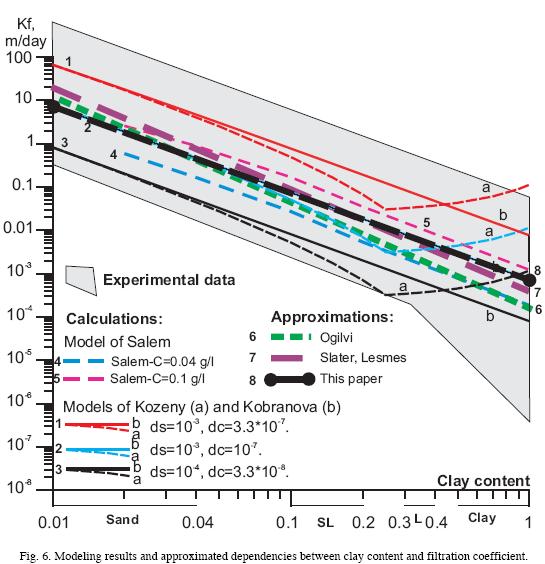
In Figure 6 we present theoretical calculations using formulas (3) and (6a) for models from Figure 4, for the formula of Sal em (1) and approximation formulas (as straight lines in logarithmic coordinates) for data of Ogilvi (9), and Slater & Lesmes (10) including approximation formula (11) for all data in Figure 6. We used straight line approximations in logarithmic coordinates to obtain formulas in the form Kf=A.C-B, where A and B are constants. Coefficient A in this formula can be calibrated by direct Kf measurements in each site.
The formulas are the following:
where C is clay content in relative units between 0.01 and 1. Formula 11 has the feature that the power exponent for clay content is equal to 2, as in Kobranova's formula.
These approximation formulas can be used for recalculation of practical clay content values into filtration coefficient values. These expressions have restrictions. Clay content should not be zero. They are only valid for clay–sand soils. Differences between Kf values calculated from formulas 9–11 should nor exceed one order of magnitude. We recommend some calibration of soil filtration coefficient at each site, when possible.
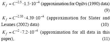
Formula (10) was obtained by using experimental data such as clay content and hydraulic conductivity estimated in the laboratory and presented in Slater and Lesmes (2002). This information allows calculating correlation between filtration coefficients measured directly and estimated from clay content (Figure 7) for different types of formations (sand, till, silt, loam, mixture of sand and clay, kaolin and bentonite) with correlation coefficient 0.79.
By means of the VES method, it is possible to estimate the filtration coefficient on base of clay content, found from soil resistivity and groundwater salinity (Shevnin et al., 2004). Finally, it is possible to calculate the hydraulic conductivity by the following steps:
(1) Geoelectrical measurements along profiles with VES method at the site. We recommend 2D Resistivity Imaging field technology of VES.
(2) 1D, or better, 2D VES data interpretation in order to find the true resistivity distribution.
(3) Recalculation of true resistivity values along with groundwater salinity into clay content, using a soil model obtained from soil sample measurements.
(4) Recalculation of clay content into filtration coefficient (hydraulic conductivity values), using one of equations
(9–11) and using results of direct Kf determination for calibration.
CLAY CONTENT ESTIMATION FROM GEOPHYSICAL DATA
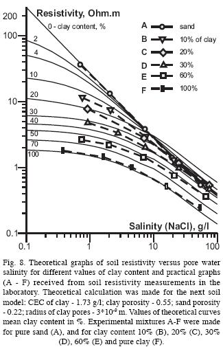
Hydraulic conductivity estimation from clay content can be practical when geophysics provides this parameter (clay content). A technique for clay content estimation from resistivity measurements was developed. The first step includes soil sampling and the measurements of soil resistivity versus pore water salinity in the laboratory (Shevnin et al., 2004). Soil curve resistivity versus water salinity is interpreted with Petrowin software (Ryjov and Sudoplatov, 1990; Shevnin et al., 2005) to estimate sand–clay model parameters, such as clay content, sand and clay porosity, and cation exchange capacity of clay. This technique was checked on soil mixtures of calibrated sand and montmorillonite clay with clay content from 0 to 100% (Figure 8). In this case, maximal error of clay content estimation was 18%. This error level leads to reliable estimation of the main lithological types of sand–clay soils, such as: sand, sandy loam, loam, clay. This technique helps obtaining a soil model of the site used in the process of VES resistivity and groundwater salinity interpretation in terms of clay content.
The second step is used for recalculation (interpretation) of soil resistivity and pore water salinity values into values of clay content, also with the help of the Petrowin program (Shevnin et al., 2005). Soil sampling in this case is used to obtain a typical soil model for the study site. This model and groundwater salinity are used to transform electric resistivity values obtained from VES data interpretation into petrophysical parameters, and first of all into clay content. We think that maximal errors of clay content estimation do not exceed 1.2–1.5 times the true clay content value. For example, for a clay content of 0.1 (10%) there will be error limits between 0.07 – 0.15 (7% – 15%). An error in clay content calculation will produce an error in hydraulic conductivity estimation. After using formulas (9 –11), an error in Kf calculation shouldn' t exceed 5–fold limits of true Kf value (at the local level), but according to Figure 5 the natural regional dispersion has 4 orders of magnitude for each clay content value. Such error can be reduced only with the help of Kf calibration at the studied site, obtained with direct hydrogeological Kf measurements.
Clay content variation between 0.01 and 1 (1 – 100%), according to Figures 5–6 produces 50 000–fold variation in Kf value. In this case the 5–fold error in Kf calculation constitutes only 1/1000 part of the total Kf range. With this level of errors, we count on the needed resolution in Kf calculation to provide real Kf value estimation within one order of magnitude or decade of logarithmic scale, in all ranges of Kf values. Thus we shall obtain an acceptable Kf estimation in the intervals 0.01–0.1; 0.1–1; 1 –10 m/d, etc., and this accuracy is sufficient to resolve many hydrogeological problems. These errors do not take into account the natural scatter in Kf. This problem can be resolved with calibration.
PRACTICAL EXAMPLES
Hydraulic conductivity estimation, developed in this paper, is based on clay content values found from VES resistivity and groundwater salinity taking into account a soil model of the site, estimated from soil sample resistivity versus salinity measurements. As for VES results, hydraulic conductivity values can be presented as cross–sections (for VES profiles, Figure 10), maps (Figure 11) or tables of parameters (Table 1).
As an example of this application, we present the site Km42, near Cárdenas, Tabasco. The cross–section includes four layers: superficial covering (layer 1), loam (layer 2), sandy aquifer (layer 3), and clay–rich basement (layer 4) (Figure 9).
We calculated the petrophysical parameters (Table 1) by using mean values of electrical resistivity for each layer, mean groundwater salinity (0.05 g/l) estimated for this site, and a soil model found from samples. There is no calibration data for Kf.
There are three cross–sections for the same profile of the site in Figure 10: resistivity cross–section obtained after 2D VES data interpretation, cross–sections of clay content and filtration coefficient. On these cross–sections it is possible to distinguish four layers from values of resistivity, clay content and filtration coefficient. The main sandy aquifer (the 3rd layer) is clearly visible from its maximum resistivity, minimum clay content and high values of filtration coefficient.
In Figure 11 three maps: electric resistivity, clay content and filtration coefficient are presented for an oil contamination site called Mecatepec, near Poza Rica, Veracruz. In the resistivity map there is a low resistivity anomaly corresponding to petroleum contamination. Low resistivity in the contaminated zone is due to the biodegradation of contaminants. This contaminated zone is shown on two other maps due to anomalous values of clay content and filtration coefficient. These anomalies allow contaminated zone mapping. Probably the clay contents and filtration coefficient values are not true in the contaminated zone, but these anomalous values allow mapping the contaminated zone both in plan and with depth, sometimes with better accuracy than with resistivity data. We think that petrophysical parameters (in this case clay content and filtration coefficient, estimated from VES data are very useful and practical for contamination mapping.
CONCLUSIONS
1. Estimation of the filtration coefficient with superficial resistivity method (VES) has an advantage in comparison with direct estimation of this parameter, because of its speed, high resolution and low cost. Direct measurements of filtration coefficient may help to calibrate indirect measurements.
2. Filtration coefficient is related to different soil parameters. Among these, in our opinion, clay content is correlated with filtration coefficient. Clay content estimation with the technology of VES survey on true resistivity, obtained from VES interpretation, groundwater salinity estimation (obtained in the field on groundwater resistivity) and soil model from soil measurements (resistivity versus pore water salinity) in laboratory, should take into account groundwater salinity and soil humidity as factors of high influence on soil resistivity.
3. Filtration coefficient of soil depends on many factors, like clay content, grain size, type of clay, anisotropy of layered sediments, and two types of capillaries in clay. As a result, dependence of filtration coefficient from clay content is scattered. The scatter can be diminished with the help of calibration by using direct Kf measurements at each site.
4. – The steps for estimation of filtration coefficient are the following:
a) VES field measurements in the area of study with 2D Resistivity Imaging technology.
b) 2D interpretation of VES data with the program Res2DInv or with similar algorithm.
c) Measurements of groundwater resistivity in all possible points of the site to estimate its salinity.
d) Soil sampling for measurements in the laboratory of resistivity versus pore water salinity, which yields a soil model used in operation (e).
e) Recalculation of two parameters (soil electrical resistivity and groundwater salinity) into clay content.
f) Recalculation of clay content into filtration coefficient with the help of formulas (9 – 11) taking into account calibration results, obtained from direct measurements of filtration coefficient, when possible.
g) Visualization of calculation results as sections and maps.
ACKNOWLEDGMENTS
We are indebted to The Mexican Petroleum Institute, where this study was performed. We thank two anonymous reviewers for their comments that significantly improved the manuscript. We thank the Editorial for the help with English corrections.
BIBLIOGRAPHY
BASSIOUNI Z., 1994. Theory, measurement, and interpretation of well logs, SPE Textbook Series Vol. No. 4, 372 p. [ Links ]
BERG, R. R., 1970. Method for determining permeability from reservoir rock properties. Trans. Gulf Coast Assoc. Geol. Soc., 20, 303–317. [ Links ]
BÖRNER, F. D., J. R. SCHOPPER and A. WELLER, 1996. Evaluation of transport and storage properties in the soil and groundwater zone from induced polarization measurements. Geophys. Prosp., 44, 583–601. [ Links ]
CLAPP, R. B. and G. M. HORNBERGER, 1978. Empirical equations for some soil hydraulic properties. Water Res. Res. 14, 601–604. [ Links ]
DE WIEST, R. J. M., 1965. Geohydrology. John Wiley & Sons, Inc. 366 p. [ Links ]
FREEZE, R. A. and J. A. CHERRY, 1979. Groundwater. Prentice Hall, Inc. [ Links ]
GAVICH, I. K., B. C. KOVALEVSKY, L. C. JAZVIN et al., 1983. Hydrogeology principles. Hydrodynamics, Novosibirsk: Nauka. 241 p. [ Links ]
EPA, 1986. http://web.ead.anl.gov/resrad/datacoll/conuct.htm , The Environmental Assessment Division (EAD) of Argonne National Laboratory. [ Links ]
GEOPHYSICAL METHODS IN HYDROGEOLOGY AND ENGINEERING GEOLOGY, 1985. Ministry of Geology of the USSR. Moscow, Nedra. 183 p. (In Russian). [ Links ]
HÖRDT, A., R. BLASCHEK, A. KEMNA, J. SUCKUT and N. ZISSER, 2005. Hydraulic conductivity estimation from spectral induced polarization data – a case history. SAGEEP–2005, 226–235. [ Links ]
KNOLL, M., R. KNIGHT and E. BROWN, 1995. Can accurate estimates of permeability be obtained from measurement of dielectric properties? SAGEEP Annual Meeting, Orlando, Florida. [ Links ]
KOBRANOVA, V. N., 1986. Petrophysics – the 2nd edition, Moscow, Nedra, 392 pp. (In Russian). [ Links ]
KONISHI, C. and G. KOBAYASHI, 2005. An interpretation of various well logs acquired in unconsolidated soil for hydraulic property estimation. SAGEEP–2005, 236–244. [ Links ]
KULCHITSKY, L. J., O. G. USYAROV, F. G. GABIBOV, 2000, Physical and chemical model of water–saturated clay and its usage at study of volumetric deformations of clay soil. Baku, 41 pp. (In Russian) [ Links ]
MAZAC, O., M. CISLEROVA, W. E. KELLY, I. LANDA and D. VENHODOVA, 1990. Determination of Hydraulic Conductivities by Surface Geoelectrical Methods. In: Geotechnical and environmental geophysics. Ed. S. Ward. [ Links ]
MARION, D., 1990. Acoustical, Mechanical and Transport Properties of Sediments and Granular Materials, Ph.D. thesis, Stanford Univ., Stanford, Calif. [ Links ]
MCKAY, L. D., 2002. Principles of hydrogeology. Course notes. Geology 485 / Civil Engineering 485. University of Tennessee. Fall.
MELKANOVITSKY, I. M., 1984. Geophysical methods in regional hydrogeological studies. Moscow, Publishing house "Nedra". 176 pp. (In Russian). [ Links ]
MIRONENKO, V. A. and V. M. SHESTAKOV, 1978. Theory and methods of interpretation of filtration field experiments. M.: "Nedra", 1978. 325 pp. (In Russian). [ Links ]
OGILVI, A. A., 1990. Fundamentals of engineering geophysics. Moscow, Nedra, 501 pp. (In Russian). [ Links ]
RYJOV, A. A. and A. D. SUDOPLATOV, 1990. The calculation of specific electrical conductivity for sandy – clayed rocks and the usage of functional cross–plots for the decision of hydrogeological problems. In: Scientific and technical achievements and advanced experience in the field of geology and mineral deposits research. Moscow, pp. 27–41. (In Russian). [ Links ]
SALEM H.S., 2000. Interrelationships among Water Saturation, Permeability and Tortuosity for Shaly Sandstone Reservoirs in the Atlantic Ocean. Energy Sources, 22, 333 – 345. [ Links ]
SALEM, H. S., 2001. Modelling of lithology and hydraulic conductivity of shallow sediments from resistivity measurements using Schlumberger vertical electrical soundings. Energy Sources, 23 (7), 599–618. [ Links ]
SHEVNIN, V., O. DELGADO RODRÍGUEZ, A. MOUSATOV and A. RYJOV, 2004. Soil resistivity measurements for clay content estimation and its application for petroleum contamination study. SAGEEP–2004, Colorado Springs. p. 396–408. [ Links ]
SHEVNIN, V., O. DELGADO–RODRÍGUEZ, L. FERNÁNDEZ–LINARES, H. ZEGARRA MARTÍNEZ, A. MOUSATOV and A. RYJOV, 2005. Geoelectrical characterization of an oil contaminated site in Tabasco, Mexico. Geofís. Int., 44, 3, 251–263. [ Links ]
SHEVNIN, V., O. DELGADO–RODRÍGUEZ, A. MOUSATOV and A. RYJOV, 2006. Estimation of soil superficial conductivity in a zone of mature oil contamination using DC resistivity. SAGEEP–2006, Seattle. P. 1514–1523. [ Links ]
SLATER, L. and D. LESMES, 2002. Electrical–hydraulic relationships observed for unconsolidated sediments. Wat. Resour. Res., 38 (10). PP.31–1 – 31–13. [ Links ]
USGS–1987. Hydrogeology, Aquifer Characteristics, and Ground–Water Flow of the Surficial Aquifer System, Broward County, Florida. Water–Resources Investigations Report 87–4034 US Department of the Interior. US Geological Survey. J. E. Fish. [ Links ]

