Estimation of soil petrophysical parameters from resistivity data: Application to oil–contaminated site characterization

 

Vladimir Shevnin¹, Omar Delgado Rodríguez¹, Aleksandr Mousatov¹, David Flores Hernández¹, Héctor Zegarra Martínez¹ and Albert Ryjov²

 

¹ Mexican Petroleum Institute, Eje Central Lázaro Cárdenas 152, 07730, Mexico D.F. E–mail: vshevnin@imp.mx

² Moscow State Geological Prospecting Academy, Geophysical faculty, Volgina str., 9, 117485, Moscow, Russia.

 

Received: May 23, 2005
Accepted: August 1, 2006

 

Resumen

El método Sondeo Eléctrico Vertical (SEV), conocido desde 1912, ha cambiado sustancialmente durante los últimos 10 años, apareciendo una nueva tecnología llamada Imagen de Resistividad (IR) con interpretación 2D de los datos de resistividad. Otra vía posible de desarrollo del método SEV es, partiendo de las relaciones existentes entre la resistividad eléctrica y los parámetros petrofísicos (PP), estimar estos últimos a partir de datos de IR. Para la realización práctica de este concepto fue desarrollada la teoría del problema directo e inverso que relaciona la resistividad eléctrica con los PP. Cada trabajo de campo deberá incluir un levantamiento de SEV (IR), mediciones de resistividad eléctrica del agua subterránea con el objetivo de determinar su salinidad y la recolección de algunas muestras representativas de suelo del sitio con mediciones hechas en laboratorio de la resistividad eléctrica como función de la salinidad del agua de poro, creando el modelo petrofísico del suelo de este sitio. Esta tecnología puede ser utilizada tanto para la caracterización de sitios limpios como contaminados por hidrocarburos. Para el caso de sitios contaminados, los valores de los PP determinados en laboratorio, salinidad de agua y los datos de IR, permiten establecer la frontera petrofísica entre suelo limpio y contaminado, y por consiguiente, configurar la pluma contaminante. En este trabajo se incluyen, como ejemplos prácticos, los resultados de la aplicación de esta tecnología en algunos sitios contaminados por hidrocarburos en México.

Palabras clave: Parámetros petrofísicos de suelo, modelación petrofísica, contenido de arcilla, porosidad, capacidad de intercambio catiónico, Sondeo Eléctrico Vertical, Imagen de Resistividad 2D, contaminación por hidrocarburos.

 

Abstract

Vertical Electrical Sounding (VES) method, known from 1912, has changed greatly during the last 10 years, into a new technology named Resistivity Imaging (RI) with 2D data interpretation. Another possible development for VES method is estimating petrophysical parameters (PP) from RI data, using the relationship between electrical resistivity and PP. In order to reach this purpose, the theory of the forward and inverse problem that relates the electrical resistivity with PP was developed. Each field survey should include a VES (RI) survey, groundwater resistivity measurements in order to determine the groundwater salinity, and collecting some representative soil samples in the study site for resistivity measurements as function of pore water salinity in laboratory, creating a soil petrophysical model of the site. This technology can be used for the characterization of uncontaminated and oil contaminated sites. For the case of contaminated site PP values determined in laboratory, groundwater salinity and RI data help to define the petrophysical boundary between contaminated and uncontaminated soil, and consequently, to obtain the contamination plume. In this work, the results of the application of this technology in some hydrocarbon contaminated sites in Mexico are presented.

Key words : Petrophysical parameters of soil, petrophysical modeling, clay content, porosity, cation exchange capacity, Vertical Electrical Sounding, 2D Resistivity Imaging, oil contamination.

 

INTRODUCTION

Vertical Electrical Sounding (VES) is a classical method of applied geophysics used for distant and nondestructive study of the upper part of geological medium. It uses direct current (DC) injected in the ground surface to investigate the underground electrical resistivity. For the last 10 – 15 years this method has changed greatly, from solution of traditional 1D model (horizontal layering) to 2D (and 3D) models for interpretation in heterogeneous media. Field technology of VES method was transformed from performance of soundings made in separated and independent points, with spacing of current electrodes growing in logarithmic scale, to measuring system with multi–electrode array distributed along profiles (known as Resistivity Imaging – RI). In the case of RI, the step between sounding sites is equal or proportional to the inter–electrode distance. For the 3D survey, the information is collected on a grid of profiles distributed on the earth surface. There are many publications on the theory of forward and inverse problem solution (including interpretation algorithms) for DC resistivity method above 2D and 3D heterogeneous media (Loke and Barker, 1995, 1996). RI technology and 2D data interpretation improved greatly the detail and accuracy of inhomogeneous media study.

At the same time there is another important possibility in VES method development. This is the relation between soil resistivity and petrophysical parameters. Well known Archie formula (Archie, 1942) displayed rock's resistivity relation with groundwater salinity, porosity and formation factor. Soil studies uncovered also the influence of humidity, volumetric clay content, grain size and packing, cation exchange capacity and contaminants on resistivity. All this knowledge allowed developing a theory of soil resistivity and algorithms of forward problem solution (calculation of resistivity using known PP) and inverse problem solution (estimation of some PP from soil resistivity, taking into account that all others PP are known or fixed).

There are many papers on electrical properties of hard rocks (mainly for oil well logging). Quantity of papers about loose soils electrical properties is noticeably less (Marion et al., 1992; Klein and Santamarina, 2003; Revil and Glover, 1998). In papers of Ryjov (1987) and Ryjov and Sudoplatov (1990) was developed algorithm of resistivity calculation for sand–clay soils, based on two–component model of soil (sand and clay).

To determine PP from resistivity one need to provide in the theory and in experiments the sufficient amount of information to develop some methodology of quantitative PP determination. Estimation of PP with VES method does not cancel traditional methods of PP determination in geological, chemical and agronomical laboratories, but can add to these some data obtained distantly, rapidly and with high spatial density. Traditional laboratory methods are accurate, but punctual and expensive. Rational integration of traditional laboratory methods and VES can provide PP estimations with higher density and lower cost in optimized time and with increasing quality.

VES method offers great advantages at oil contamination studies. Oil contaminants cause series of changes in physical, chemical and biological properties of soil (Modin et al., 1997; Sauck, 1998; Atekwana, 2001), mainly during first several months after contamination. Just after contamination a high resistivity anomaly marks contaminated zone, but after several months, as a result of biodegradation of contaminants under the influence of bacteria, this zone reveals a low resistivity anomaly.

Sauck (1998) in his contamination model proposed that low resistivity anomalies in mature contaminated sites resulted in an increase of salt content in pore water. According to Sauck, low resistivity is created by intense bacteria action on petroleum products and chemical interactions of contaminants and their products with soil grains in a lower part of vadose zone. In this model, bacteria, through biodegradation, produce organic and inorganic acids increasing the dissolution of minerals and releasing the ions that increase the levels of total dissolved solids (TDS) in pore water.

The model of Sauck was modified by Atekwana et al. (2001; 2003), and Abdel Aal et al. (2004). Atekwana et al. (2003) found that there is no tight correlation between soil and water resistivity in contaminated zones, so, another cause of low resistivity anomaly should be found. Abdel Aal et al. (2004)  explained that the main cause of low resistivity anomaly is superficial conductivity increase in soil pores compared with electrolytic conductivity. Resulting process is reflected in apparent changes of PP estimated from soil resistivity.

Shevnin et al. (2005a) found that, in the case of clean soil, PP values estimated from resistivity are close to real values, but in oil contaminated zones PP becomes anomalous. For example, in contaminated zone, clay content estimated from resistivity (it is called quasi–clay) seems increased noticeably. Electrical conductivity in clay resulted in superficial conductivity and this conductivity increases in contaminated soil due to biodegradation products. That is why increasing quasi–clay is found.

The basic principle of petrophysical interpretation consists in analysis of relation between soil resistivity and pore water salinity. To estimate clay content, porosity and cation exchange capacity from soil resistivity, finding or fixing all other PP values as much as possible close to reality is needed. To find them representative soil samples are collected in the site and their resistivity as function of water salinity ρ(C) is measured. This curve ρ(C) is interpreted to find such PP as sand porosity, clay capillary radii, clay content and clay CEC. These parameters can be used as a petrophysical model in interpretation of soil resistivity and pore water salinity to estimate clay content, porosity and CEC of soil.

 

VES METHOD WITH RI TECHNOLOGY

Apparent resistivity (ρ_a) pseudo–section (Figure 1A), which is a result of RI technology, can be interpreted in terms of 2D model (Loke and Barker, 1995, 1996), giving a true or soil resistivity (ρ) cross–section (Figure 1B). 2D model consists of rectangular cells reaching infinitely in the horizontal direction perpendicular to the profile. All cells have the same vertical thickness in one depth interval. That is why such level can be considered as a layer (not as a real geological layer, but some model layer). Number of layers and their thicknesses are fixed for the whole site. RI technology in this paper was applied to study the soil structure until 10 – 20 m deep. In this case geological sections are mainly horizontally–layered (consist of different geological layers) or pseudo–layered ρ(z) structures (due to the influence of groundwater level and weathering). In both cases physical properties change more in vertical, than in lateral direction. In this situation 2D interpretation (with Res2DInv) increases the inversion quality due to more correct accounting of near–surface and deep inhomogeneities' influence, and regularization in inversion process makes its results more stable.

Traditional result of 1D interpretation is a horizontally layered model with layers spreading infinitely in lateral directions. Nevertheless during nearly one century 1D results were used to study 2D and 3D geological structures on a grid of VES. 2D interpretation gives more stable geological results along each profile and it can be also used to study 3D structures, especially in a situation with nearly horizontal layering. With some restrictions an assumption can be made that 2D interpretation gives information about some ρ(z) distribution (restricted volume instead of infinite horizontal prisms) below each VES point, all VES being distributed on the site area along profiles. In case of cells with vertical thickness 1 m, soil volume for resistivity determination amounts several cubic meters. These assumptions are suitable for pseudo–layered models and allow creating a soil resistivity cube (Figure 2) (Shevnin et al., 2005a) for an easy preparation of vertical sections for any profiles and horizontal maps (lateral ρ changes) for some fixed depths.

Theoretically evident solution to use 3D inversion algorithms is not practical. Existent algorithms of 3D interpretation give unstable solutions or need to apply very detailed and complicated 3D field survey. Now more practical solution is to make 2D interpretation for each profile in the study site and then to create 3D model in spite of all restrictions of this approach.

 

PETROPHYSICAL INTERPRETATION OF SOIL RESISTIVITY

The important step in VES method improvement is petrophysical interpretation of soil resistivity. This technology was developed by A. Ryjov (Ryjov, 1987; Ryjov and Sudoplatov, 1990) and then applied in Mexico at more than 12 sites with oil contamination (Ryjov and Shevnin, 2002; Shevnin et al., 2004; 2005a, b; 2006). The forward petrophysical problem consists in the calculation of soil resistivity values on the base of PP of some soil model (mixture of sand and clay). The inverse problem consists in PP estimation on the base of soil resistivity and pore water salinity, taking into account petrophysical soil model of the site. For practical realization of petrophysical interpretation in each site it is necessary to obtain VES data, groundwater salinity and representative soil samples to measure their resistivity versus pore water salinity in laboratory and then to interpret data creating soil model of the site.

The basic model for loose soils is the sand and clay mixture. Grain sizes of sand and clay differ in four orders. If clay content is less than sand porosity smaller clay particles are situated in greater sand pores. When clay content is more than sand porosity, sand grains are dispersed in clay matrix. Sand and clay capillaries are completely (or partially) filled with water. Clay capillaries radii are comparable with electric double layer (EDL) thickness. As a result, clay conductivity is formed under the EDL influence. Sand capillaries radii are much greater than EDL thickness, and EDL does not influence on sand conductivity.

An example of the forward petrophysical problem solution, (that is theoretical resistivity calculation for a given soil model) is presented in Figure 3A. Soil resistivity curves for different sand and clay proportions are here displayed: the curve for clean sand (in the upper part of Figure 3 A, 0% of clay) and the curve for pure clay (in the lower part of Figure 3A, 100% of clay). This model curves were calculated for pore radii in sand 10^–4 m, in clay 10^–8 m, sand porosity 0.25, clay porosity 0.55, CEC of clay 3 g/l and full water saturation of soil pore space. Figure 3B shows theoretical dependence of porosity from clay content for the model A. Porosity curve begins at 25% (sand porosity), has minimum when clay content is equal to sand porosity and all sand pores are filled with clay, and then increase until clay porosity (55%). Left part of curve was formed under the influence of sand porosity, while the right part is influenced by clay content and clay porosity.

Theoretical curve for sand resistivity vs water salinity (Figure 3, curve 0) is practically straight line situated in parallel and above water resistivity curve. These curves decline of straight lines at high salinity (near solubility limit). The clay and clay–sand mixture curves at high salinity (more than 5 g/l) are situated in parallel to the lines for sand and water with distribution along vertical axis according to soil porosity. The curves for clay and clay–sand mixture for salinity less than 5 g/l are not in parallel to the lines for sand and water, cross water curve and their vertical distribution depends on clay content. Such non–linear behavior of the curves for clay – rich soil resulted in clay EDL and CEC influence.

An important peculiarity of sand and clay resistivity should be commented: their difference depends on water salinity. When water salinity is 0.01 g/l, sand to clay resistivity ratio is equal to 780, for salinity 0.1 it is equal to 80, for salinity 1 it is equal to 10 and for salinity 10 it is equal to 3 (Figure 3).

So, resolution of resistivity method to differentiate soil lithologies depends on groundwater salinity and decreases with salinity increasing.

This also shows that clay content determination on soil resistivity cannot be performed without knowledge of pore water salinity.

 

INTERPRETATION OF SOIL SAMPLES RESISTIVITY MEASUREMENTS AS FUNCTION OF WATER SALINITY

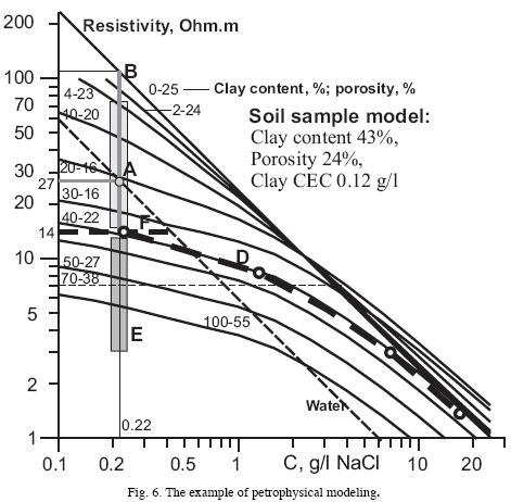
Representative soil samples collected in each site are dried and homogenized in a laboratory. The soil is distributed into 4–5 resistivimeters (with volume about 200 ml each) and filled until full saturation with NaCl solutions having salinity in interval 0.5 – 50 g/l with the step 2–3 times. Experimental resistivity curve ρ(C) (see example in Figure 6) is interpreted by fitting with theoretical curves calculated for petrophysical model (sand and clay capillary radii, porosity, formation factor and CEC of clay). Some model parameters can be adjusted during interpretation. Final best–fit model gives clay content in soil, soil porosity and adjusted sand and clay components parameters. This soil model is then used for soil resistivity (obtained from VES) and groundwater salinity petrophysical interpretation.

In Figure 4 there are graphs of errors in soil PP estimation as a function of fitting error for the case of soil samples measured in laboratory. Fitting error is the RMS error between experimental and theoretical ρ(C) curves. Errors were estimated with the help of statistical approach, developed by Goltsman (1971) and Tarantola (1994). Errors in clay content estimation are 6–17% when fitting error is 2–5%. Experimental studies of calibrated soils in laboratory gave us mean error in clay content estimation equal to 18% (Shevnin et al., 2006).

Sand and clay curves from Figure 3 are displayed in Figure 5 as groups of curves. Each group is presented by series of curves depending on sand porosity, and clay CEC.

The sand curve depends closely on the sand porosity (Figure 5). Unlike the sand, clay porosity changes are not so high. Montmorillonite (bentonite) counts on 60% porosity, kaolin – 50% and hydromica – 55%. There is another factor that influences on clay resistivity: CEC of clay. Clay line position in Figure 5 depends on CEC. That is why a soil resistivity model of the site is needed for petrophysical interpretation.

 

CATION EXCHANGE CAPACITY (CEC)

Clay and organic matter particles act as giant anions, with their surface covered with a net of negative charges. Cations are attracted to the surface and exchange takes place. CEC is simply a measure of the quantity of sites on the soil grains surface that can retain positively charged ions (cations) by electrostatic force. The electrostatically retained cations are easily exchanging with other cations in soil pore solution. The cations exchange sites are mainly located on clay grains surface. Normal range of soil CEC is in interval from <4 meq/100g (for sandy soil) to >25 meq/100g (for rich – clay soil). Increase of organic material in soil notably increases CEC.

 

AN IDEA OF CLAY CONTENT, POROSITY AND CEC DETERMINATION ON VES RESISTIVITY

Knowing soil resistivity and pore water salinity, it is possible (with the help of Figure 3 A) to estimate clay content, and then to estimate soil porosity from clay content by using Figure 3B.

Let's consider the situation when sand–clay soil resistivity is 10 Ohm.m and water salinity is 0.01 g/l. In this case, clay content estimated on Figure 3A is 30% and porosity found on Figure 3B is 15%. If salinity is equal to 1 g/l for the same soil resistivity, clay content would be 20% and porosity found from clay content would be 16%. In uncontaminated sites clay CEC is the same for the whole area. Clay CEC is determined in laboratory by measuring and interpreting soil resistivity vs salinity curve. The soil CEC depends on clay content in soil and clay CEC of the site and it can be determined in this way from resistivity values.

 

RELATION BETWEEN CONTAMINATED ZONE AND LOW RESISTIVITY ANOMALY

When a leakage of light non–aqueous phase liquids (LNAPL) takes place, it penetrates into subsoil, changing its physical – chemical properties, electrical resistivity between them. The resistivity difference between contaminated and clean soil depends on such factor as the age of contamination event. In case of recent leakage, the contaminated soil creates high resistivity anomalies, being generally proportional to a contamination level. On the other hand, when the leakage is aged (from four months to a year after the contamination, or more) oil contamination creates low resistivity anomalies.

The main factors that influence on clay sand mixture resistivity are the following: clay content, water salinity and conductivity, clay and sand capillaries structure. Mature oil contamination slightly increases water solution conductivity, changes pore structure by filling pores with biodegradation products and changes superficial conductivity in pores (Abdel Aal et al., 2004). This effect on soil resistivity is equivalent to the increase of clay content that can be found in the clay content estimation process and used as criteria to discriminate oil contaminated zones.

 

PETROPHYSICAL MODELING FOR MATURE OIL CONTAMINATED SITE

Petrophysical modeling consists in some analysis of information for each site (soil resistivity from VES, soil samples resistivity curve ρ(C) and its petrophysical model, and water salinity), in order to compare all information and estimate its consistency. All information obtained is displayed on the template with coordinates: soil resistivity – water salinity (Figure 6). The template itself is calculated for a soil model obtained from soil curves–ρ(C) interpretation. This interpretation gives clay and sand parameters (porosity, capillary radii, clay CEC) and clay content in soil. Template in Figure 6 was calculated for clay CEC 0.12 g/l, sand porosity 0.25, clay porosity 0.55. Each theoretical curve is marked with clay content and soil porosity. There is also experimental curve for soil sample–ρ(C) (Line D). Groundwater resistivity of this site is 27 Ohm.m. Horizontal line 27 Ohm.m crosses water curve in the point with salinity 0.22 g/l, so water salinity is determined. All possible soil resistivity values of this site (at complete water saturation) are on this line – 0.22 g/l. This soil sample is typical for clean soil of the site and shows clay content 43%. From geological data maximum clay content is in the first layer and should not be more than 43 %, but there are some soils here with less clay content until pure sand. This information helps to conclude that all soils resistivities of the site are in interval 14–110 Ohm.m, from soil with 43% of clay until pure sand (along line B). Boundary F of minimum soil resistivity of the area is equal to 14 Ohm.m. Statistical distribution of soil resistivity values of the site has values in the areas A and E. This site was contaminated by oil well many years ago. Mature oil contamination gives low resistivity anomalies. From petrophysical modeling it can be concluded that soil with resistivity below the boundary value 14 Ohm.m corresponds to contaminated soil. A clay content exceeding 43% (for soil resistivity below the boundary F) is obtained in soil resistivity interpretation with PP estimation. For soil resistivity interpretation between 3 and 5 Ohm.m clay CEC value should be increased, because 100% clay with CEC=0.12 g/ l can not give resistivity below 5 Ohm.m. Low resistivity in the area was created by oil contamination, so clay content in soil more than 43 % is indicator of contamination and does not show real increase of clay content. This effect is called quasi–clay. Such petrophysical modeling is performed for each site.

 

PRACTICAL EXAMPLE : MECATEPEC–3, VERACRUZ

The results of 2D resistivity interpretation in terms of PP for the site Mecatepec–3, Veracruz are presented in Figure 7. Four maps were obtained for the 3rd layer of 2D interpretation with depth from 2 to 3 m. It shows that petrophysical parameters (Figures 7 B–D) of the contamination plume traced similar zones as the soil resistivity anomaly does (Figure 7A).

Bold line in each map means boundary between clean and contaminated soil. Boundary value was estimated through petrophysical modeling by integration of groundwater salinity, soil resistivity, and soil petrophysical characteristics (clay content, porosity and CEC). Boundary values (separating clean and contaminated soils) were estimated for resistivity equal to 10 Ohm.m, for clay content – 80%, for porosity – 46%, for CEC – 0.5 g/l.

 

PRACTICAL EXAMPLE: KM124, TABASCO

Site Km124 was contaminated as a result of a spill from the pipeline. This site is in sandy soil with low clay content (<10%). Groundwater level, at the moment of the resistivity study was at a depth of 2.5 m, but it changes from 1 to 4 m deep due to annual changes in precipitation, as well as the influence of a pond nearby and the high hydraulic conductivity of the soil. As a result, contaminated soil smeared with oil was found in a depth interval from 1 to 3 m. The main problem with VES data from this site was interpretation of soil resistivity and groundwater salinity in terms of petrophysical parameters in conditions of vadose zone (incomplete water saturation) with noticeable changes of humidity. To perform this operation, soil samples were collected in different parts of the site and clay content and CEC were found by means of laboratory measurements of resistivity vs salinity curves and its interpretation. Clay content was below 10%. Then theoretical dependencies of soil resistivity from clay content and humidity were calculated (Figure 8A) by using Ryjov's algorithm (Ryjov and Sudoplatov, 1990). After 2D interpretation of the VES data, the mean soil resistivity distribution (Figure 8B) and then clay content and humidity distribution with depth (Figures 8C, 8D) were found.

Which is the best form of VES data visualization, through sections or maps? Visualization in sections has less interpolation distance between measuring points. To create maps a distant interpolation between profiles is necessary. However maps have lower resistivity range than sections (electrical properties change more with depth than in plan) (Figure 9). As a result in maps visualization a higher resolution can be reached with the possibility of some weaker anomalies locating. To adjust resistivity range a statistical analysis was applied, allowing to increase visualization resolution (Figure 9, Table 2) and scale range. Without special adjustment of resistivity range it is frequently not possible to locate oil contamination anomalies on sections and maps. In case of aged contamination resistivity ratio between clean and contaminated soil is from 2 to 5. To locate contamination anomaly, maximum resolution of visual presentation is needed and it is easier to obtain in case of maps. Both sections and maps help us to have an idea of contamination distribution in space.

Algorithm of Ryjov was created for soil resistivity interpretation in terms of petrophysical parameters for all data with equal soil humidity. For data interpretation in the vadose zone a separate interpretation for different layers needs to be used, each layer counting on its own humidity.

Thus, resistivity interpretation in terms of petrophysical parameters for each layer obtained in 2D VES interpretation is performed taking into account soil humidity. Soil resistivity map for the second layer (0.7–1.6 m depth) is displayed in Figure 10. Petrophysical maps for this layer have a similar outline of the contaminated zone. Boundary line for the second layer separating clean and contaminated soil (Figure 10) is equal to 170 Ohm.m.

Two months before resistivity survey at the Km124 site, measurements of soil gases were performed to detect concentrations of volatile organic compounds (VOC). Soil resistivity and VOC values have correlation coefficient –0.62 and their dispersion is shown in Figure 11. When VOC increasing (reflecting growth of contamination grade) resistivity decreasing about 5 times.

Two superposed maps of clay content (estimated from resistivity) and VOC concentrations are presented in Figure 12. Anomalies in these maps are congruent despite of the fact that data for both maps were measured in different time periods and with different grids. It is necessary to note that clay content anomaly actually resulted into an increase of superficial conductivity in contaminated soil (Abdel Aal et al., 2004). Borehole 2 was drilled at the point with the highest VOC value and detected free product at a depth of 1.5 m and groundwater level at 1.6 m.

 

CONCLUSIONS

Resistivity Imaging technology along with 2D interpretation (with Res2DInv software) is a very useful instrument for shallow 3D study with creating soil resistivity cube and presenting results in sections or maps for different layers.

To obtain maximum resolution of visualization, sufficient for contaminated zones localization, layers maps are more suitable.

Interpretation of resistivity values in terms of petrophysical parameters means a step forward in geological characterization of uncontaminated and oil contaminated sites, studied by means of resistivity method.

 

ACKNOWLEDGMENTS

We are indebted to The Mexican Petroleum Institute, where this study was performed. We thank anonymous reviewers for their comments that significantly improved the manuscript.

 

Bibliography

ARCHIE, G. E., 1942. The Electric Resistivity Logs as an Aid in Determining some Reservoir Characteristics. SPE–AIME Transactions, 146, 54–62.        [ Links ]

ABDEL, AAL, G. Z., E. A. ATEKWANA, L. D. SLATER, and E. A. ATEKWANA, 2004. Effects of microbial processes on electrolytic and interfacial electrical properties of unconsolidated sediments. Geophys. Res. Lett., 31, 12, L12505 10.1029/2004GL020030        [ Links ]

ATEKWANA, E., D. P. CASSIDY, C. MAGNUSON, A. L. ENDRES, D. D. WERKEMA, JR and W. A. SAUCK, 2001: Changes in geoelectrical properties accompanying microbial degradation of LNAPL. In: Proceedings of the Symposium on the Application of Geophysics to Engineering and Environmental Problems. 1 – 10.        [ Links ]

ATEKWANA, E. A., E. A. ATEKWANA and R. S. ROWE, 2003. Relationship Between Total Dissolved Solids and Bulk Conductivity at a Hydrocarbon–Contaminated Aquifer, SAGEEP Proceedings, pp. 228–237.        [ Links ]

BOBACHEV, A.A., 1994. IPI2Win software: http://geophys.geol.msu.ru/rec labe.htm        [ Links ]

BOBACHEV, A.A., 2003. X2IPI software: http://geophys.geol.msu.ru/x2ipi/x2ipi.html         [ Links ]

GOLTSMAN, F. M., 1971. Statistical models of interpretation. Moscow., 328 pp. (In Russian).        [ Links ]

KLEIN, K. A. and J. C. SANTAMARINA, 2003. Electrical conductivity in soils: Underlying phenomena. J. Environ. Engin. Geophys., 8, 4, 263–273.        [ Links ]

LOKE, M. H. and R. D. BARKER, 1995. Least–squares deconvolution of apparent resistivity pseudosections. Geophysics, 60, 1682–1690.        [ Links ]

LOKE, M. H. and R. D. BARKER, 1996. Rapid least–squares inversion of apparent resistivity pseudosections using a quasi–Newton method.Geophys. Prospect., 44, 131–152.        [ Links ]

MARION, D., A. NUR, H. YIN and D. HAN, 1992, Compressional velocity and porosity in sand–clay mixtures. Geophysics, 57, 554–563.        [ Links ]

MODIN, I. N., V. A. SHEVNIN, A. A. BOBATCHEV, D. K. BOLSHAKOV, D. A. LEONOV and M. L. VLADOV, 1997. Investigations of oil pollution with electrical prospecting methods. 3rd Meeting environmental and engineering geophysics. Proceedings. Aarhus, Denmark, 8–11 September 1997. p.267–270.        [ Links ]

REVIL, A. and P. W. J. GLOVER, 1998. Nature of surface electrical conductivity in natural sands, sandstones, and clays. Geophys. Res. Lett., 25, 5, 691–694.        [ Links ]

ROWELL, D. L., 1993. Soil science: methods and applications. Longman Scientific and Technical. P. 133. ISBN 0–470–22141–0        [ Links ]

RYJOV, A., 1987. The main IP peculiarities of rocks. In: "Application of IP method for mineral deposits' research". Moscow, 1987, 5–23. (In Russian).        [ Links ]

RYJOV, A. and V. SHEVNIN, 2002. Theoretical calculation of rocks electrical resistivity and some examples of algorithm's application. In: Proceedings of the Symposium on the Application of Geophysics to Engineering and Environmental Problems.        [ Links ]

RYJOV, A. A. and A. D. SUDOPLATOV, 1990. The calculation of specific electrical conductivity for sandy – clayed rocks and the usage of functional cross–plots for the decision of hydrogeological problems. In: "Scientific and technical achievements and advanced experience in the field of geology and mineral deposits research. Moscow, pp. 27–41. (In Russian).        [ Links ]

SAUCK, W. A., 1998. A conceptual model for the geoelectrical response of LNAPL plumes in granular sediments. In: Proceedings of the Symposium on the Application of Geophysics to Engineering and Environmental Problems, 805–817.        [ Links ]

SHEVNIN, V., O. DELGADO RODRÍGUEZ, A. MOUSATOV and A. RYJOV, 2004, Soil resistivity measurements for clay content estimation and its application for petroleum contamination study. SAGEEP–2004, Colorado Springs. p. 396–408.        [ Links ]

SHEVNIN, V. , O. DELGADO–RODRÍGUEZ, A. MOUSATOV, H. ZEGARRA MARTÍNEZ, J. OCHOA VALDÉS and A. RYJOV, 2005a. Study of petroleum contaminated sites in Mexico with resistivity and EM methods. SAGEEP Proceedings, Atlanta, Georgia, pp. 167–176.        [ Links ]

SHEVNIN, V., O. DELGADO RODRÍGUEZ, L. FRENÁNDEZ–LINARES, H. ZEGARRA MARTÍNEZ, A. MOUSATOV and A. RYJOV, 2005b. Geoelectrical characterization of oil contaminated site in Tabasco, Mexico. Geofís. Int., 44, 3, 251–263.        [ Links ]

SHEVNIN, V., A. MOUSATOV, A. RYJOV and O. DELGADO, 2006. Estimation of clay content in soil based on resistivity modeling and laboratory measurements. Geophysical Prospecting. In print.        [ Links ]

TARANTOLA, A., 1994. Inverse problem theory. Method for data fitting and model parameter estimation. Elsevier Science, Amsterdam, 600 p.        [ Links ]