


Servicios Personalizados
Revista
Articulo
 Inglés (pdf)
 Artículo en XML
 Referencias del artículo
 Enviar artículo por email
Indicadores
-
 Citado por SciELO
 -
 Accesos
Links relacionados
-
 Similares en
SciELO
Similares en
SciELO
Compartir

 Permalink
Geofísica internacional
versión On-line ISSN 2954-436Xversión impresa ISSN 0016-7169
Geofís. Intl vol.45 no.3 Ciudad de México jul./sep. 2006
Faulting process and coseismic stress change during the 30 January, 1973, Colima, Mexico interplate earthquake (Mw=7.6)
Miguel A. Santoyo, Takeshi Mikumo and Luis Quintanar
Instituto de Geofísica, UNAM. Ciudad Universitaria, 04510, México D.F., México. Email:masantoyo@correo.unam.mx
Received: May 20, 2005
Accepted: September 5, 2006
Resumen
El 30 de enero de 1973 ocurrió un evento mayor de subducción (Mw=7.6) en la interfase de las placas de Cocos y Norteamérica, cerca del punto triple entre las placas de Rivera, Cocos y Norteamérica. Este evento podría estar relacionado con dos secuencias de grandes sismos subsecuentes que ocurrieron alrededor de esta región. Aunque varios autores han analizado el mecanismo focal y la profundidad de este sismo, nosotros analizamos las características de la fuente y realizamos una inversión cinemática lineal de la distribución de deslizamientos sobre el plano de falla a través del modelado de forma de onda. Encontramos un mecanismo inverso (St=285°, Dip=16°, Ra=85°) consistente con la tectónica regional, con una profundidad de 16 km y una liberación total de momento de 2.98x1027 dyn–cm. Los resultados muestran una distribución de deslizamiento con dos manchas principales, con una dislocación máxima de 199 cm y 173 cm respectivamente. Este sismo rompió dos asperezas principales en el plano de falla extendido: una en la parte inferior y al suroeste y la otra en la parte superior y al noroeste del hipocentro, con un cambio de esfuerzos de –31 y –40 bars respectivamente. El área circundante de incremento de esfuerzo podría haber influenciado la sismicidad subsecuente a una distancia de hasta 120 km del hipocentro.
Palabras clave: Cambio de esfuerzo cosísmico.
Abstract
A large thrust earthquake (Mw=7.6) occurred on January 30, 1973, on the plate interface between the subducting Cocos plate and the continental North America plate, near the triple junction between the North America, Cocos and Rivera Plates. This event might be related to two sequences of subsequent large earthquakes that occurred around this region. Although several authors have analyzed the focal mechanism and depth of this earthquake, we analyzed its source characteristics and performed a linear kinematic waveform inversion for the slip distribution over the fault plane. We find a shallow thrust mechanism (St=285°, Dip=16°, Ra=85°) consistent with the tectonic environment, with a depth of 16 km and a total moment release of 2.98x1027 dyn–cm. The results show a slip distribution with two main patches, with a maximum dislocation of 199 cm and 173 cm respectively. We calculated the coseismic stress change on and around the fault plane. This earthquake ruptured two main asperities, one downdip and southwest and the other updip and northwest of the hypocenter, with stress change of –31 and –40 bars respectively The surrounding zone of stress increase could have influenced the subsequent seismicity to a distance of up to 120 km from the hypocenter.
Key words: Coseismic stress change.
INTRODUCTION
The northwestern portion of the Mexican subduction zone is a rather complicated tectonic region. High seismic activity is directly related to subduction of the Rivera and Cocos oceanic plates under the North America plate (Figure 1). The Rivera plate is a relatively small plate with a convergence rate of 2.5 cm/year relative to North America (DeMets et al., 1994), which has produced some of the greatest earthquakes in the last century, such as the 3/06/ 1932, Ms=8.2 and 18/06/1932, Ms=7.6, Jalisco earthquakes (Singh et al., 1985) and the 9/10/1995, Mw=8.0, Colima–Jalisco earthquake (Pacheco et al., 1997). Although the southeastern edge of this plate is uncertain, it may be limited by a triple junction near El Gordo Graben (EGG), which could also limit the Cocos plate (Figure 1) (Kostoglodov and Bandy, 1995). The Cocos plate, on the other hand, has higher convergence rates with respect to North America than the Rivera plate, ranging between 5.2 cm/year near its northwest edge (Figure 1) to 8.2 cm/year near the Tehuantepec ridge at the southeastern portion of the Mexican subduction zone (DeMets et al., 1997). Subduction of the Cocos plate is also responsible for large and great thrust earthquakes such as the 29/11/1978, Mw=7.8, Oaxaca earthquake and the 19/09/1985, Mw=8.1, Michoacán earthquake (Singh and Mortera, 1991), and some large normal–faulting events (e.g. the 11/1/1997, Mw=7.1, Arteaga earthquake and the 30/09/1999, Mw=7.5, Oaxaca event) (Santoyo et al., 2005a, Singh et al., 2000).
Recent studies have revealed the possibility of stress interaction between large–thrust and inslab normal–faulting earthquakes (Mikumo et al., 1999; Mikumo et al., 2002), and among large–thrust interplate events in this subduction zone (Mikumo et al., 1998; Santoyo et al., 2005b). In order to discuss a seismic recurrence cycle and the associated seismic hazard in Mexico, a detailed study of large earthquakes and their postseismic activity is indispensable.
The earlier 30 January 1973 (Mw=7.6) earthquake was a low–angle thrust event that ruptured the interface between the North–America plate and the northwestern edge of Cocos plate. Its epicenter (–103.21°E, 18.39°N; Lomnitz, 1977) was located inland close to the EGG and the diffuse triple junction near the Rivera plate (Figure 1). A previous event occurred in April 15, 1941 very close to the 1973 event (102.94°W, 18.85°N) with a similar magnitude (Ms=7.8). Two subsequent major seismic events were located northwest (the 9/10/1995 Colima–Jalisco and 22/01/2003 Tecomán earthquakes; Santoyo et al, 2005b), and another four occurred to the southeast (the 25/10/1981 Playa Azul, 19/ 09/1985 Michoacán, 21/09/1985 Zihuatanejo and 14/03/ 1979 Petatlán earthquakes; Santoyo et al., 2005b). These shocks have been studied by different authors from a finite fault point of view (Figure 2). A detailed study of the 1973 event and its associated coseismic stress change is essential to look for a possible spatial and temporal relation between these two large seismic sequences and to improve our knowledge of the seismicity and the state of stress in the region.
Several authors have studied different point source characteristics of the 1973 earthquake. Lomnitz (1977) located the mainshock epicenter with the aid of a distance residual algorithm, using the P arrival times recorded at 254 local and teleseismic stations. His results show a location error of less than 5 km for the epicenter (–103.21 °E, 18.39°N) with a source depth of 32 km. Reyes et al. (1979) obtained a focal mechanism solution (strike=330°, dip=30°, rake=65°) for a source depth of 35 km, based on the P wave polarities in regional and teleseismic recordings. They also studied the epicentral distribution of 2–week aftershock activity, and concluded that the earthquake most probably occurred on the interface between the Cocos and North America plates. Chael and Stewart (1982) also studied the source properties and obtained a different solution (strike=266°, dip=17°, rake=55°) with a source depth of 20 km. To constrain the vertical plane they used P wave first motion arrival data from Mexican stations, mainly with compressional arrivals and only one dilatational observation. They don't mention which stations are used in this case. To constrain the shallow dipping plane of the focal mechanism, they used spectral amplitudes from WWSSN of the R3 arrivals at 200 s, obtained from Reyes et al., (1979). These data were mainly used to estimate the Rayleigh wave radiation pattern. Peak amplitudes then were plotted as a function of the azimuth and were compared with synthetic radiation patterns. By this comparison Chael and Stewart obtained the focal mechanism. In any case, they didn't model the waveforms for this event because they inferred a complex source.
Singh and Mortera (1991), using the seismograms from station DBN (DeBilt, Holland), obtained a rather complex source time function composed of several subevents, all located at a shallow depth of 8 km. They mention, however, that this result appears somehow unusual in contrast to neighboring events, especially the 15/04/41 earthquake where the source time function is much simpler than for the 1973 event. Pardo and Suárez (1993) described the geometry of the Benioff zone in the region, finding that the angle of plate subduction changes from 8° near the trench to about 30°, 300 km away from the trench. Their finding suggests that the dip of the interface at the location of the 1973 event is of about 17° at a depth of 21 km. Finally, based on the mechanism obtained by Chael and Stewart, Quintanar (1991) obtained a spatial distribution of the seismic moment release using an iterative inversion method proposed by Kikuchi and Kanamori (1982) and later extended by Kikuchi and Fukao (1985). From this distribution, he found a main patch downdip from the epicenter and two other pathches southeast and northwest of the nucleation point.
The objective of this work is to obtain reliable focal information, to perform a detailed finite fault inversion for the spatial distribution of slip, and to compute the associated coseismic stress change over the plate interface. To do this, we based our analysis on teleseismic P waveform seismograms recorded at different WWSSN stations.
DATA
We examined the LPZ P waveform arrivals recorded on 8 WWSSN digitized analog seismograms, with a sampling interval of 0.5 sec. Only teleseismic stations located between 30° and 90° were considered in order to avoid the distorted P waves that propagate inside the earth's upper mantle and through the earth's outer core respectively. These stations are listed in Table 1, and as it can be seen here, they have a wide azimuthal coverage.

The recordings were corrected for the instrumental response, filtered with a three–pole low–pass butterworth filter (fc=0.33 Hz) and integrated into displacement time histories.
POINT SOURCE CHARACTERISTICS
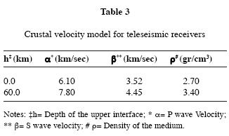
As described before, different focal mechanisms and depths have been obtained from previous studies for this earthquake. As a first step, we performed a point source inversion for the main focal properties and depth. To do this, we inverted the teleseismic displacement waveforms, using the Nábêlek's (1984) maximum–likelihood inversion technique. The crustal velocity model used for the source region is that adopted by Santoyo et al. (2005a) for the Michoacán region (Table 2). A global crustal velocity model shown in Table 3 was used for the teleseismic receivers. Here we also included the attenuation parameter t* of 1.0 second for P waves (Futterman, 1962).

To obtain the main focal characteristics, we first fixed the source depth at 20 km, and performed a linear inversion for the focal mechanism, source time function and total moment release. After the inversion, the focal mechanism solution obtained was found to be: strike=285°, dip=16° and rake=85°, a total moment release of 2.98x1027 dyn–cm, and a total duration of 26 sec for the source time function. This solution is similar to that obtained by Chael And Stewart (1982). In Figure 3 we show the solution, together with a comparison between the observed records (solid lines) and the synthetic seismograms (dashed lines). The focal mechanism and the relative location of the teleseismic stations are shown on the lower focal hemisphere. For the estimation of the best source depth we performed an RMS error analysis fixing the above parameters, computing the synthetic seismograms for different source depths, and comparing them with the observations. Figure 4a shows the results from this analysis where we obtained a minimum RMS error at a depth of 16.5 km. After this procedure was done, we performed a global inversion for the focal mechanism and the source depth. Doing this, we obtained a very similar solution. For the estimation of the best dip angle we also made a similar analysis. In Figure 4b we show that a dip angle of 15° to 17° yields the lower RMS relative error.
FAULTING PROCESS
Once the main point source characteristics were estimated, we performed a finite fault inversion for the slip distribution over the fault plane. The method of waveform inversion used in this study was originally developed by Hartzell and Heaton (1983) and has been applied successfully to several Mexican earthquakes (e.g. Mendoza and Hartzell, 1989; Mendoza, 1993, 1995; Courboulex et al., 1997; Santoyo et al., 2005a). For the inversion, we assumed that the fault plane is the plate interface with a strike of 285°and a dip of 16° to the northeast. Here, we assumed a fault area of 145 km by 85 km in the strike and dip directions, respectively, based on the aftershock distribution obtained by Reyes et al. (1979), and discretized it into 493 square subfaults of equal size (5 km x 5 km), which are embedded in the horizontally layered structure of Table 2. The hypocenter was located at the center of the fault plane (–103.21°E, 18.39°N) at a depth of 16 km. The fault dimensions thus assumed cover the depths between 5 and 27 km.
Synthetic seismograms are then calculated for each pair of subfaults and teleseismic stations, applying the generalized ray theory proposed by Helmberger (1974) and Langston and Helmberger (1975) for teleseismic distances. The point–source responses (Green's functions) are shifted by the time delay corresponding to the rupture propagation from the hypocenter. We assumed here a constant rupture velocity that implies circular rupture fronts centered at the nucleation point or the hypocenter. The responses of each subfault are calculated for a triangular source time function of a given duration (STFD), which was assumed the same for all the subfaults on the fault plane.
Based on this assumption, the observed data together with the synthetic seismograms form an over–determined linear system of the type AX≈B . Here, the matrix A contains the synthetic seismograms with their respective time shifting due to the rupture delay, B is a vector with the observed records arranged in the same order as in the synthetics in matrix A, and X is the solution vector containing the dislocation weighting values which represent the amount of slip that must be applied to each subfault in order to fit the observations.
The matrix equation shown here can be solved by a simple least–squares technique; however, the solution could become unstable if matrix A is ill–conditioned (Hartzell and Heaton, 1983). To solve this problem, the inversion was stabilized by a Householder decomposition of the matrix equations (Lawson and Hanson, 1974; Menke 1984), imposing a positivity constraint to the solution. To further stabilize the inversion, we appended, to the linear system, additional smoothing and moment–minimization constraints of the form λFX =λD , where λ is a scalar weighting factor. Smoothing is imposed by constructing F and D such that the difference between adjacent dislocations be zero. Moment minimization is obtained by letting F be the identity matrix and D the zero vector, effectively reducing the length of X . To identify the proper weighting factor λ, several inversion runs are conducted until the largest value of X is reached that still allows the observed records to be fit by the synthetic waveforms. In this case, spatial smoothness constraints are imposed to reduce some noise effects included in the solution, which could come from some unconsidered path effects or simplification of the velocity model.
For this inversion we used the velocity recordings instead of the displacement data at the 8 mentioned stations, mainly because these waveforms supply more information in high frequencies than the displacement seismograms, which allow us to obtain a better spatial resolution on the slip distribution.
To estimate the values of the STFD and rupture velocity that best fit the observations, we performed several inversion runs, varying the STFD between 2.0 sec and 3.0 sec and the rupture velocity between 2.5 km/sec and 3.5 km/sec. Due to the inherent trade–off between these two unknowns, the value for the STFD was obtained as a function of the rupture velocity to have a smooth rupture along the fault. After this analysis, we observed that a rupture velocity of 2.7 km/sec and a source time function duration of 2.5 sec for each subfault, produced a more coherent solution and better fit between the observed and synthetic seismograms.
In order to assure the reliability of the source depth already estimated, we also performed an additional RMS analysis for the source depth, based on the finite source inversion. In this case we computed the synthetic seismograms and performed several inversion runs for different depths of the fault plane. We show in Figure 5 the results from this analysis, having a minimum RMS error for a source depth of 17 km. From these results, we conclude that a source depth between 16 and 17 km is a reliable value.

The inversion results using the above parameters show the best agreement between the synthetic and observed velocity seismograms (Figure 6). The dislocation pattern is shown in Figure 7. Slips are shown in cm and the black star shows the hypocenter location on the fault plane. The "x" axis represents the length in the horizontal (strike) direction and the""y" axis represents the width in the dip direction. From the slip distribution obtained, it can be observed that the rupture produced two main patches: One of them 20 km downdip from the hypocenter with a maximum slip of 199 cm, and the other one updip and southeast of the hypocenter, with a maximum slip of 173 cm. The total moment release obtained from this inversion is 2.78x1027 dyne–cm, with an overall source time function duration of 26 sec, and a roughly triangular shape with some small high–frequency small variations on the seismic moment release (Figure 8).

COULOMB FAILURE STRESS CHANGE
The 30/01/1973 earthquake occurred near the triple junction region where the oceanic Cocos and Rivera plates subduct beneath the continental North America plate. This event may have some spatial relations to different earthquake sequences that occurred a few tens of years later, one on the Rivera plate interface and the other one on the Cocos plate interface (Figures 1 and 2). To investigate this possible relation, we estimate the coseismic stress change inside the fault area of this earthquake, and also the spatial extent of the stress influence of this earthquake over the two plate interfaces.
Taking into account the final slip distribution, we calculated the coseismic change of the Coulomb failure stress function  due to this earthquake. To do this, we computed the Coulomb failure stress from the relation
  (e.g. Harris, 1998), where Atis the shear stress change in the direction of the fault slip,
  is the change in the tensional stress normal to the fault plane, and ¡x'is an apparent coefficient of friction μ' = μ(1–p), where μ is the static coefficient of friction and p is the pore pressure in the source volume.
All these stresses were calculated in a tensorial way for a 3D model using the formulations given by Okada (1985, 1992). In the computations, we used the mean shear modulus for the site, μ=3.5 x l011 dyn/cm2, with a Poisson ratio of v=0.25. For the tectonic apparent coefficient of friction, we used the value of μ'=0.4 adopted by Mikumo et al. (2002) for the Mexican subduction zone. Based on the extent of the fault area of this earthquake we take, for the computation of the stress, a rectangular plate interface covering an area of 300 km by 275 km on the strike and dip directions respectively. Here, we used a mesh size of 2.0 km x 2.0 km for the location of the computation points.
Figure 9 show the Coulomb failure stress change for this earthquake over the extended fault plane, resolved in the same plane and in the slip direction. Here, the "x" axis (abscissa) represents the distance along the strike direction, which is approximately parallel to the coast, and the "y" axis (ordinate) represents the distance in the dip direction also indicating the depth. Contours are given in bars. The black star shows the hypocenter on the fault plane. It can be observed in this figure that the earthquake ruptured two main asperities: One downdip and northwest of the hypocenter with a maximum stress change of –31 bars and a total length of about 100 km in the horizonthal direction, and the other updip and southwest of the hypocenter with a maximum stress change of –40 bars and a similar size of the first one. There are also two zones of stress increase with a maximum vaue of 25 bars inside the fault area, and also stress increase zones extending to the surrounding fault area.
DISCUSSION AND CONCLUSIONS
Previous studies by different authors on the source characteristics of this earthquake differ in fault geometry, focal depth and source time function duration. We believe that our results show a tectonically consistent focal mechanism and source depth. Our focal mechansism agrees with the tectonic setting and the geometry of the Benioff zone described by Pardo and Suárez (1993) for the region. Our estimated source depth using two different RMS error analyses is based on a point source and finite fault inversions. In both cases, the minimum RMS error occurs at 16–17 km depth, suggesting that previous source depths of this event were underestimated (Singh and Mortera, 1991) and overestimated (e.g Reyes et al., 1979). Also the source time functions obtained by previous authors show different durations and complexities. Quintanar (1991) obtained a simple triangular source time function with a 27 sec duration, and Singh and Mortera (1991) obtained a rather complex source time function. Our results mainly show a simple function with some high frequencies and a duration of 26 sec.
The difference between our source time function and the one obtained by Singh and Mortera (1991) could be explained by different assumptions in the computation of synthetics and in the number of waveforms analyzed. They used a simple homogeneous half–space earth model over the source region, while we used a multi–layered model appropriate to the region. In this case, the complexities in the wave train usually produced by a layered earth and recorded on the seismogram at the DBN station, which is the only station they used, could have been attributed to the source.
Numerous studies have shown that there is a positive correlation between the zones of coseismic stress increase inside and around the source region due to a large earthquake and the increment of subsequent seismicity in these regions (Reasenberg and Simpson, 1992; King et al., 1994; Deng and Sykes, 1997; Stein et al., 1997; Harris, 1998, Stein, 1999). Some of these studies suggested possible triggering of a large earthquake due to previous events with similar magnitudes. In addition, it has been suggested that stress increases as small as 0.1 bars could influence subsequent seismicity in the surrounding region of a ruptured fault (e.g. Deng and Sykes, 1997; Stein, 1999).
If we assume an increment of 0.5 bars in the Coulomb stress to have an effective influence on subsequent events, the stress increase zone sourounding the fault area should reach about 1.5 times the length and two times the width of the fault area. This event could therefore have an effective influence on subsequent events at a distance as far as 120 km from the hypocenter.
ACKNOWLEDGMENTS
Carlos Mendoza kindly provided some codes for the inversion procedures. Synthetics for teleseismic distances were computed based on the program TELEDB by Charles A. Langston. The Coulomb failure stress computations were performed using the code DIS3D by Laurie Erickson. We thank Jaime Yamamoto for his suggestions on the WWSSN stations. This work was partially supported by the CONACYT project No. 41209–F.
Due to the limitations of the data set used for the computation of slips, we performed three different analyses to overcome this deficiency.
Analysis for the low–pass cut frequency on the slip pattern
Here we performed the kinematic inversion based on the same observed seismograms low–pass filtered with a cut frequency of Fh=.125 Hz. The results are compared with respect to the original filtered data (Fh=.33). In Figures A1a and A1b we show the fit between data and synthetics using the new filter, and the corresponding slip pattern. It can be observed that the slip pattern changes in some way but the general pattern is maintained. This shows that high frequencies on the seismograms are not necessarily controlling the details of the slip distribution.
Resolution analysis for the slip distributions superimposing white noise on seismograms
In an effort to overcome the deficiency of S wave information, we performed a resolution analysis. Here we superimposed white noise of different amplitudes on the observed data and performed the inversion for slips. In Figures A2a–A2h of Appendix we show the slip distribution obtained for each amount of noise superimposed to the observations. Figure A3 shows the RMS errors for each amount of noise. It can be observed that after 2% of noise, the slip pattern begins to change.
Comparison between the "De Bilt" station with respect to the STU (WWSSN) station
The "De Bilt" station DBN record was not included because its location on the focal mechanism is very similar to the other European stations. To show that the information contained in this particular station is similar to other stations close to this one on the focal sphere, we deconvolved the vertical P wave arrival for the instrumental response of the Galitzin–Willip seismograph and compared it with station STU. In Figure A4 we show the result of the deconvolution analysis and in Figure A5 we compare this waveform with the one recorded at the station Stutgart (STU) for the same event. As it can be observed, the waveform of the DBN station is almost identical to the time history at the STU station.
BIBLIOGRAPHY
CHAEL, E.P. and G.S. STEWART, 1982. Recent large earthquakes along the Middle American trench and their implications for the subduction process. J. Geophys. Res. 87, 329–338. [ Links ]
COURBOULEX, F., M. A. SANTOYO, J. PACHECO and S. K. SINGH, 1997. The 14 September 1995 (M=7.3) Copala, Mexico earthquake : A Source study using teleseismic, regional, and local data. Bull. Seism. Soc. Am. 87, 999–101. [ Links ]
DEMETS, C., R. GORDON, D. ARGUS and S. STEIN 1994. Effect of recent revisions to the geomagnetic reversal time scale on estimates of current plate motions. Geophys. Res. Lett. 21, 20, 2191– 2194. [ Links ]
DEMETS, C. and D. S. WILSON, 1997. Relative motions of the Pacific, Rivera, North American, and Cocos plates since 0.78 Ma. J. Geophys. Res., 102, 2789–2806. [ Links ]
DENG J. and L.R. SYKES, 1997. Evolution of the stress field in southern California and triggering of moderate–size earthquakes: A 200–year perspective. J. Geophys. Res., 102, 9859–9886. [ Links ]
FUTTERMAN, W. I., 1962. Dispersive body waves. J. Geophys. Res. 67, 5279–5291. [ Links ]
HARRIS, R., 1998. Introduction to special section: stress triggers, stress shadows, and implications for seismic hazards. J. Geophys. Res., 103, 24347–24358. [ Links ]
HARTZELL S. H. and T. H. HEATON, 1983. Inversion of strong ground motion and teleseismic waveform data, for the fault rupture history of the 1979 Imperial Valley, California, earthquake. Bull. Seism. Soc. Am., 76, 1553–1583. [ Links ]
HELMBERGER, D., 1974. Generalized ray theory for shear dislocations. Bull. Seism. Soc. Am., 64, 45–64. [ Links ]
KING, G. C. P., R. S. STEIN and J. LIN, 1994. Static stress changes and the triggering of earthquakes. Bull. Seism. Soc. Am. 84, 935–953,. [ Links ]
KIKUCHI, M. and Y. FUKAO, 1985. Iterative deconvolution of complex body waves from great earthquakes: The Tokachi–Oki earthquake of 1968. Phys. Earth Planet. Interiors, 37, 235–248. [ Links ]
KIKUCHI, M. and H. KANAMORI, 1982. Inversion of complex body waves. Bull. Seism. Soc. Am., 72, 491–506. [ Links ]
KOSTOGLODOV, V. and W. BANDY, 1995. Seismotectonic constraints on the convergence rate between the Rivera and North American plates. J. Geophys. Res., 100, 17,977–17,989.D [ Links ]
LANGSTON, C. and D. HELMBERGER, 1975. A procedure for modelling shallow dislocation sources. Geophys. Journ. Roy. Astr. Soc., V. 42, 117–130. [ Links ]
LAWSON C. L. and R. J. HANSON, 1974. Solving least squares problems. Ed. Prentice Hall Inc., Englewood Cliffs, New Jersey, 340p. [ Links ]
LOMNITZ, C., 1977. A procedure for eliminating the indeterminacy in focal depth determination. Bull. Seism. Soc. Am., 67, 533–535. [ Links ]
MENKE, W., 1989. Geophysical data analysis: Discrete inverse theory. Ed. Academic Press Inc., San Diego, CA., USA, 289p. [ Links ]
MENDOZA and HARTZELL, 1989. Slip distribution of the 19 September 1985 Michoacán, Mexico, earthquake: Near source and teleseismic constraints. Bull. Seism. Soc. Am. 79, 655–669. [ Links ]
MENDOZA, 1993. Coseismic slip of two large Mexican earthquakes from teleseismic body waveforms: Implications for asperity interaction in the Michoacán plate boundary segment. J. Geophys. Res., 98, 8197–8210. [ Links ]
MENDOZA, 1995. Finite fault analysis of the 1979 March 14, Petatlán, Mexico earthquake using teleseismic P waveforms. Geophys. J. Int., 121, 675–683. [ Links ]
MENDOZA and HARTZELL, 1997. Fault slip distribution of the 1995 Colima–Jalisco, Mexico, earthquake. Bull. Seism. Soc. Am., 89, 1338–1344. [ Links ]
MIKUMO, T., T. MIYATAKE and M. A. SANTOYO, 1998. Dynamic rupture of asperities and stress change during a sequence of large interplate earthquakes in the Mexican subduction zone. Bull. Seism. Soc. Am. 88, 686–702. [ Links ]
MIKUMO, T., S. K. SINGH and M. A. SANTOYO, 1999. A possible stress interaction between large thrust and normal faulting earthquakes in the Mexican subduction zone. Bull. Seism. Soc. Am. 89, 1418–1427. [ Links ]
MIKUMO, T., M. A. SANTOYO and S. K. SINGH, 2000. Dynamic rupture and stress change in normal faulting earthquakes in the subducting Cocos plate. Geophys. J. Int., 140, 611–620. [ Links ]
MIKUMO, T., Y. YAGI, S. K. SINGH and M. A. SANTOYO, 2002. Coseismic and postseismic stress changes in a subducting plate: Possible stress interactions between large interplate thrust and intraplate normal faulting earthquakes. J. Geohys. Res., 107, B1, ESE5–1–ESE5–12. [ Links ]
NABELEK, J. L., 1984. Determination of earthquake source parameters from inversion of body waves. PhD. dissertation, Massachusetts Institute of Technology, Cambridge, Mass. [ Links ]
OKADA, Y., 1985. Surface deformation due to shear and tensile faults in a half space. Bull. Seism. Soc. Am. 75, 1135–1154. [ Links ]
OKADA, Y., 1992. Internal deformation due to shear and tensile faults in a half space. Bull. Seism. Soc. Am. 82, 1018–1040. [ Links ]
PACHECO, J., S. K. SINGH, J. DOMÍNGUEZ, A. HURTADO, L. QUINTANAR, Z. JIMÉNEZ, J. YAMAMOTO, C. GUTIÉRREZ, M. A. SANTOYO, W. BANDY, M. GUZMÁN and V. KOSTOGLODOV, 1997. The October 9, 1995 Colima–Jalisco, Mexico, earthquake (Mw 8): An aftershock study and a comparison of this earthquake with those of 1932. Geophys. Res. Lett., 24, 2223–2226. [ Links ]
PARDO, M. and G. SUÁREZ, 1993. Shape of the subducted Rivera and Cocos plates in southern Mexico: Seismic and tectonic implications. J. Geophys. Res., 100, 12357–12373. [ Links ]
QUINTANAR, L., 1991. Tomographie de la source sismique par inversion des ondes P télésismiques. PhD. dissertation, Université Paris 7, Paris, France. [ Links ]
REASENBERG, P. A. and R. W. SIMPSON, 1992. Response of regional seismicity to the static stress change produced by the Loma Prieta Earthquake, Science 255, 1687–1690. [ Links ]
REYES, A., J. N. BRUNE and C. LOMNITZ, 1979. Source mechanism and aftershock study of the Colima, Mexico earthquake of January 10, 1973. Bull. Seism. Soc. Am., 69, 1819–1840. [ Links ]
SANTOYO, M. A., S. K. SINGH and T. MIKUMO, 2005a. Source process and stress change associated with the 11 January, 1997 (Mw=7.1) Michoacan, Mexico, Inslab Earthquake. Geofís. Int., 44,4, 317–330. [ Links ]
SANTOYO, M. A., T. MIKUMO and C. MENDOZA, 2005b. Possible Lateral Stress Interactions in a Sequence of Large InterplateThrust Earthquakes on the Subducting Cocos and Rivera Plates. Submitted to Geofís. Int. [ Links ]
SINGH, S. K., L. PONCE and S. P. NISHENKO, 1985. The great Jalisco, Mexico, earthquakes of 1932: Subduction of the Rivera plate. Bull. Seism. Soc. Am. 75, 1301–1313. [ Links ]
SINGH, S. K. and F. MORTERA, 1991. Source–time functions of large Mexican subduction earthquakes, morphology of the Benioff zone, and the extent of the Guerrero gap. J. Geophys. Res. 96, 21487–21502. [ Links ]
SINGH, S. K., M. ORDAZ, L. ALCANTARA, N. SHAPIRO, V. KOSTOGLODOV, J. PACHECO, S. ALCOCER, C. GUTIERREZ, R. QUAAS, T. MIKUMO and E. OVANDO, 2000. The Oaxaca earthquake of September 30, 1999 (Mw=7.5): A normal faulting event in the subducted Cocos plate. Seism. Res. Lett., 71, 67–78 [ Links ]
STEIN, R. S., A. BARKA and J. DIETERICH, 1997. Progresive failure of the north Anatolian fault since 1939 by earthquake stress triggering, Geophys. J. Int. 128, 594–604. [ Links ]
STEIN, S., 1999. The role of stress transfer in earthquake occurrence, Nature, 402, 605–609. [ Links ]

