Prograde Rayleigh–wave motion in the valley of Mexico

 

Peter G. Malischewsky Auning¹, Cinna Lomnitz², Frank Wuttke³ and Rodolfo Saragoni⁴

 

¹ Friedrich–Schiller–Universität Jena, Institut für Geowissenschaften, Jena, Germany Email: p.mali@uni-jena.de

² Instituto de Geofísica, UNAM, México Email: cinna@prodigy.net.mx

³ Bauhaus–Universität Weimar, Bodenmechanik, Weimar, Germany Email: frank.wuttke@bauing.uni-weimar.de

⁴ Departamento de Ingeniería Civil, Universidad de Chile, Santiago, Chile Email: rsaragon@ing.uchile.cl

 

Received: March 2, 2006
Accepted: June 18, 2006

 

Resumen

El movimiento prógrado de la partícula para ondas Rayleigh en un modelo simple de una capa sobre un semiespacio se estudia teórica y experimentalmente para el caso general y para las condiciones específicas en el valle de México, D. F. Se calculan sismogramas teóricos para un modelo simplificado de la red de Texcoco. Para el sismograma de las estaciónes TACY, CU01 y SXVI del 19 septiembre de 1985 se obtiene movimiento prógrado de Rayleigh dentro de un rango de frecuencias. Los parámetros críticos para la existencia de movimiento progrado son el módulo de Poisson en la capa superficial y el contraste de velocidades de ondas S entre la capa y el semi–espacio. Para valores altos de estos parámetros el rango de movimiento progrado se encuentra aproximadamente entre la frecuencia del sitio y el doble de la misma. Adicionalmente, la zona de movimiento progrado también se presenta en dependencia en estos parámetros críticos. El estudio del movimiento de la partícula rinde constreñimiento adicional invirtiendo parámetros de modelo de las observaciones de las ondas superficiales en general y H/V estudios en especial.

Palabras clave: Ondas de Rayleigh, movimiento prógrado de la partícula, valle de México.

 

Abstract

A theory of prograde particle motion of Rayleigh waves for a layer over a half–space is derived and compared with observations in the valley of Mexico. We compute synthetic seismograms for a simplified model of the Texcoco site. The earthquake of 19 September 1985, M 8.1, featured prograde motion of Rayleigh waves within a specific frequency band. The critical parameters for the existence of prograde motion are Poisson's ratio in the layer and the shear–wave contrast between the layer and the half–space. For high values of these parameters the range of frequencies featuring prograde motion falls approximately between the site frequency and twice the site frequency. Particle motion can provide additional constraints for the inversion of surf ace–wave observations and H/V studies.

Key words: Rayleigh waves, prograde particle motion, valley of Mexico.

 

Lo menos que podemos hacer, en servicio de algo, es comprenderlo.
José Ortega y Gasset

 

INTRODUCTION

Rayleigh waves are vector waves with vertical and horizontal components that feature elliptical particle motion. Retrograde particle motion is well–established for propagation of the fundamental mode over a homogeneous half–space (Aki and Richards, 2000). In the case of an inhomogeneous half–space retrograde or prograde motion is possible, depending on the frequency range. Early papers dealing with this subject include Giese (1957) and Kisslinger (1959). Both found evidence of prograde Rayleigh motion in soils. Giese considered prograde and retrograde wave groups for a model consisting of a layer on a rigid half–space and obtained Poisson's ratio in the layer from the frequency where particle motion changes from prograde to retrograde. A recent treatment can be found in Tanimoto and Rivera (2005), who provide the eigenfunctions of Rayleigh waves and their ratios numerically for a layer over a half–space. They found that Rayleigh–wave particle motion can become prograde near the surface when the geological section contains a sedimentary layer with extremely slow seismic velocities. Prograde Rayleigh–wave motion in a layered half–space was also obtained in theory by Wuttke (2005).

Observations of prograde Rayleigh waves in the valley of Mexico were reported by Gómez–Bernal (2002) and Lomnitz and Meas (2004). Malischewsky and Scherbaum (2004) presented exact expressions for the H/V ratio in increasingly complex structures. Malischewsky et al. (2005) showed that prograde Rayleigh motion is not necessarily limited to models containing low–velocity sedimentary layers. A structural model consisting of a layer over a half–space is a convenient starting–point for developing a theory on prograde Rayleigh–wave motion. In this paper we discuss the case of the valley of Mexico, and we leave a more general rigorous analysis for a forthcoming paper.

 

THE H/V RATIO

There is a close connection between particle motion and H/V ellipticity of Rayleigh waves. Polarization is strongly frequency dependent for Rayleigh propagation in heterogeneous media. In terms of seismic hazard assessment the characterization of this frequency dependence can have important practical implications. H/V spectral ratios of ambient vibrations are increasingly used in investigations of local site amplification during strong earthquakes, as ambient noise is dominated by Rayleigh waves (Scherbaum et al., 2003; Bard, 1998). Earthquake signals can also be analyzed with the H/V method (Zschau and Parolai, 2004; Munirova and Yanovskaya, 2001). Polarization of seismic waves was analyzed by using continuous wavelet transforms (Diallo et al., 2006). These authors describe a method for detecting the switching frequency between prograde and retrograde motion. However, we show that connecting this frequency only with the peak in the H/V spectral curve is an oversimplification.

 

AN EXACT EXPRESSION FOR H/V AND PROGRADE MOTION

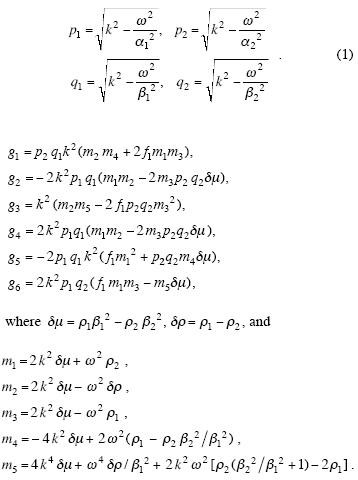
In order to obtain an exact expression for the ratio H/V in Rayleigh waves for a layer over a half–space we must first solve the corresponding eigenvalue problem, so that the phase velocity c or the wave number k can be known for a given angular frequency ω. The expression holds for all modes but we discuss the fundamental mode only. Let α₁ and β₁ be the P– and S–wave velocities in the layer,α₂ and β₂ the corresponding velocities in the half–space, ρ₁ and ρ ₂ the densities, v_l and v ₂ Poisson's ratios, and d the thickness of layer 1. We adopt the following definitions (Malischewsky and Scherbaum, 2004):

We define a quanity y as follows:

We the radio χ = H/V may be written as:

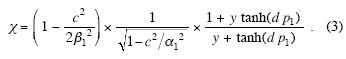
The derivation of this formula is algebraically cumbersome and lengthy. It may be found in Malischewsky and Scherbaum (2004). A famous paper by Love (1911) had treated this problem for incompressible media. A shortened explanation follows. We represent the solution of the equation of motion in terms of plane waves for the layer and the half–space, respectively. The general solution for the layer contains four integration constants, but for the half–space it has only two constants. These six constants are obtained from a system of equations, whose determinant yields the secular equation for the phase velocity of Rayleigh waves, which is assumed to be solved. Love's artifice for obtaining a reasonable analytical expression for the ellipticity was expressing the four layer constants in terms of the two half–space constants, using the continuity relations between the layer and the half–space. In this manner we obtain four equations which express the four layer constants in terms of the two half–space constants. These four equations are introduced into the two stress–free equations of the surface of the layer, which now contain only the two half–space constants. As the H/V ratio depends also on these two constants, one of the stress–free conditions can be used to eliminate one of the remaining constants and eq. (3) follows.

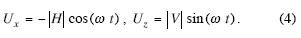
This expression enables us to obtain the particle motion. Let the eigenfunctions be defined as in Malischewsky and Scherbaum (2004), so that the horizontal component U_z is real and the vertical component U is imaginary. Omitting the imaginary unit and assuming harmonic motion, it follows from geometry (see Figure 1) that the motion is prograde for negative values of H/V :

Note that the theoretical expressions for the H/V spectrum of surface waves (Arai and Tokimatsu, 2004) are valid for any number of layers over the half–space. However, the critical dependence on the elastic parameters is hidden in an expression which follows from a computer program based on Haskell's method. It is not simply applicable in our analytical considerations. A dissertation by Bonnefoy–Claudet (2004) contains a discussion on the sense of elliptical Rayleigh motion as a function of the shear–wave contrast between layer and half–space. Wathelet (2005) discusses the numerical difficulties which are inherent in any representation of the ratio H/V.

 

H/V FOR A SIMPLIFIED TEXCOCO STRATIGRAPHY

The Texcoco array (Flores–Estrella, 2004; Stephenson and Lomnitz, 2005) is an example of a site on soft ground within the valley of Mexico. We assume a one–layer structure (Table 1), which will be later modified to bring out the essential features in our calculation.

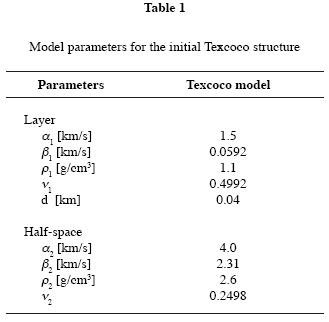
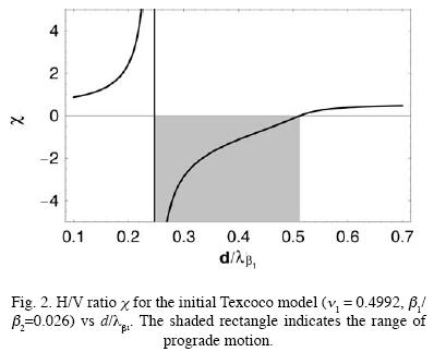
Note the extremely high Poisson's ratio v_l = 0.4992 for the layer. This value is typical for the lake–bed zone of the valley of Mexico (Stephenson and Lomnitz, 2005). It causes the range of possible prograde motion to become very significant. However, as we will see in Figure 3, such high values of Poisson's ratio are not necessary for producing prograde motion. Prograde motion may not be as rare as is often assumed.

The behaviour of the function χ is tricky, and determining some ranges of prograde motion may be a numerical challenge (Figure 2). The range of prograde motion may be bounded by two zeroes in χ ,two poles, or more commonly a pole and a zero. The latter case is displayed in Figure 2, where the range of prograde motion is indicated by a shaded rectangle.

We may now derive the behaviour of χ = H/V from Eq. (3). The 2D graph (Figure 3) shows the region of negative χ–values, or prograde motion, in red, and the region of positive χ–values or retrograde motion in blue. The abscissa is the normalized frequency where is the wavelength of shear waves in the layer. The ordinate is the ratio between the shear–wave velocities in the layer and the half–space. The calculation was carried out by using a MATHEMATICA® program.

In constructing Figure 3 we have gone beyond the initial Texcoco model in order to demonstrate the existence conditions for prograde motion. The calculation was carried out with values of v₁=0.4992, 0.4, 0.3, 0.25, 0.24, 0.23, 0.22 and 0.21. The shear–wave velocity of the layer was held constant at β₁ = 0.0592 km/s and Poisson's ratio in the half–space was assumed to be v₂ = 0.2498. The ratio of shear–wave velocities r_s = β₁ / β₂ was made to vary from 0.01 to 0.9. The value r_s = 0.026 corresponds to the initial Texcoco model (yellow horizontal line near the bottom). Malischewsky et al. (2005) showed numerically that a domain of prograde motion is also obtained for higher values of the shear–wave velocity in the layer. Thus the shear–wave velocity in the layer is not the only leading parameter for the occurrence of prograde Rayleigh motion. It must be considered in combination with Poisson' s ratio and the shear impedance contrast. The corresponding theoretical results haven been presented elsewhere but have not yet been proved analytically.

The red area in Figure 3 represents the region of prograde motion for our initial Texcoco model, as well as for the lower Poisson's ratios in the layer. The figure was calculated with the ContourPlot command of MATHEMATICA® and it may contain some random numerical noise.

Each contour required about 10 hours of computer time on a Personal Computer with 1.8 GHz timing frequency.

Other programming languages may be better suited for numerical calculations and may be more efficient.

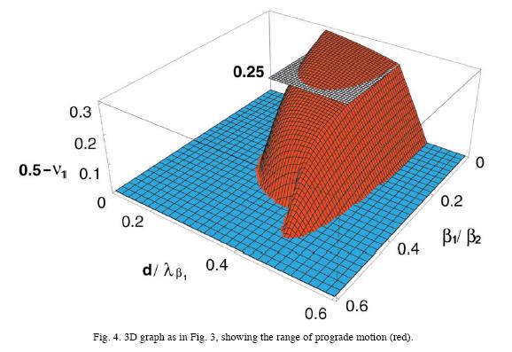
A better insight into the structure of prograde ground motion as a function of Poisson's ratio may be obtained from a 3D perspective graph (Figure 4). The contours for different values of v₁ are shown and the vertical z–coordinate is 0.5 – v₁. The red surface of this relief structure is the boundary between prograde and retrograde motion and the contours are the same as in Figure 3. The gray plane denotes v₁ = 0.25.

 

SYNTHETIC SEISMOGRAMS

Prograde particle motion is reflected in the synthetic seismograms of surface waves. For harmonic excitation the frequency range of prograde particle motion can be exactly determined (see Malischewsky et al. 2005). In the case of measured earthquake or arbitrary impulse signals it will be complicate to show the prograde particle motion. The reason is that the prograde particle motion exists only in a very short frequency range between ranges of retrograde particle motion. However the determination of this prograde particle motion in measured seismograms can be very important because the presence of prograde ground motion is related to the dominant site frequency. This raises important questions in earthquake engineering, e.g. tuning of the natural frequency of the structure by structural components far of the site frequencies.

The synthetic theoretical seismograms in this paper are computed for a single force, excited by a Ricker impulse of first order, applied to the surface of the half–space. It is useful to consider the eigenfunctions of the Texcoco site as defined in Table 1. We plot some eigenfunctions in the relevant frequency range (Figure 5). For different frequencies the horizontal (solid) and vertical (dotted) eigenfunctions are presented. Note that for frequencies higher than the site frequency β₁/4d the top layer is a waveguide.

In the range between the site frequency β₁/4d and the double site frequency β₁/2d there are changes of sign in the eigenfunctions at the top (at point β₁/4d – the horizontal eigenfunction and at point β₁/2d –the vertical eigenfunction). This is the reason for the occurrence of prograde motion in the following investigation. It must appear and ought to be observed in the calculated time histories. The calculation assumes that the wave field consists of a single mode, the fundamental mode of the site (see Figure 7b).

When the fundamental mode is used in calculations, the specific behaviour of the site in the relevant frequency range must also be reflected in the Green's functions (Figure 6) as well as in the seismograms (Figure 7). Actually the complex and the absolute values of the vertical and horizontal displacements in this frequency range are very different. This behaviour will be important for the H/V investigation of time histories.

Several techniques were used in order to check the synthetic seismograms. Figure 7b shows the results of wave field transformation, to extract the dispersion from the computed wave field in Figure 7a. For comparison, both the synthetic (dashed) and the extracted dispersion curves are plotted in Figure 7b.

There are different methods for detecting prograde ground motion in measured or calculated seismograms. Time windows may be used in the interpretation of ground motion, but often these methods are not satisfactory. Information on the polarization of the wave field is obtained in this paper by using a moving window with an appropriate window length. In Figure 8 and 9 consecutive snapshots are imaged.

The images show the expected frequency range and the corresponding prograde particle motion. The frequency content of the time window is also imaged. In Figure 8 the snapshot is early in the seismograms (t = 1.025 ... 2.825 s). Prograde ground motion only is seen in the upper window. The frequency content in this figure is in the range of 0.2 to 0.7 Hz. With increasing time Figure 9 (t = 3.85...5.65 s) shows the crossover from prograde to retrograde ground motion.

Finally we consider the H/V ratio extracted from the synthetic seismograms. The ratio is plotted in Figure 10. The ratio shows exactly the peak point at the beginning of the range of prograde particle motion at 0.37 Hz (this point is conform with the change in sign of the horizontal displacement in Figure 5 and the point β₁/4d ). The root of the ratio function appears at the frequency 0.74 Hz (point β₁/2d) and is conform to the end of the frequency range of prograde particle motion. The end of the frequency range of the prograde particle motion is caused by the change in sign of the vertical particle motion at the top of the half–space.

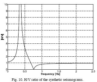
This case shows that the peak of the H/V ratio can be associated with prograde particle motion when using the Texcoco site profile. However, the occurrence of prograde particle motion depends also on the impedance ratio between the layers.

 

SOME OBSERVATIONS OF PROGRADE PARTICLE MOTION

Earthquake observations in the valley of Mexico go back to the Aztecs (García Acosta and Suárez Reynoso, 1996). Here we discuss some modern observations of Rayleigh waves, especially those with prograde ground motion. Engineering seismologists still disagree on whether Rayleigh waves or shear waves are mainly responsible for the severe damage, especially in the disastrous earthquake of 19 September 1985 in Mexico City. There are suggestions that prograde Rayleigh motion may be especially hazardous for buildings (Lomnitz and Meas, 2004). The literature about destructive seismic motion in the valley of Mexico is very substantial. Some recent references include Chávez–García and Bard (1994), Cárdenas–Soto and Chávez–García (2006), Lomnitz and Castaños (2006), and Flores–Estrella et al. (2006). Gómez–Bernal and Saragoni (1998) observed Rayleigh waves with retrograde motion in different period ranges in the valley, and the dissertation by Gómez–Bernal (2002) contains specific evidence on the 1985 event which we present here in support of our new theoretical findings. This study is not very well–known and it attempts to investigate different directions of particle motion in different period ranges in the valley. Unfortunately, Gómez–Bernal (2002) shows no example of particle motion within the lake–bed zone (Z–III). The locations of stations are shown on Figure 11. Station TEAC (18.618 N, –99.453 W) falls outside the valley in a southwesterly direction. Figure 11 shows the horizontal accelerograms and the zoning according to the Mexico City building code: Z–I (rock zone), Z–II (transition zone), and Z–III (lake–bed zone).

Figure 12 shows the vertical and radial displacement seismograms in the time window AB in order to obtain the particle motion. The top of Figure 12 shows some seismograms after bandpass filtering between 0.065 Hz and 0.15 Hz together with the extracted particle motion (retrograde). The lower section of the figure shows the same data after bandpass filtering between 0.2 Hz and 0.5 Hz plus the extracted particle motion (prograde). There is some indication that the extracted particle motion belongs to Rayleigh waves in both cases. This may agree with a model consisting of at least one layer over a half–space. Note that the retrograde motion for low–frequency waves is influenced by the half–space and the prograde motion for higher frequencies is influenced by the layer as well as the half–space.

Station SXVI shows, in the higher frequency range, prograde motion with an extremely flat ellipse, as expected from theory, which predicts this behaviour near the edges of the range of prograde motion. As station SXVI is in the transition zone (Figure 11), we assume a layer thickness of 20 m instead of the value from the Texcoco model (Table 1), and we increase the shear–wave velocity to 110 m/s, which yields a site frequency of 1.37 Hz. Twice the site frequency is about 2.75 Hz which is close to one corner frequency of the bandpass.

The high–frequency prograde motion at CU01 and TACY is more difficult to explain. For these two stations the presence of a layer is mandatory despite the accepted geological model for zone Z–I (rock site). A 25 m deep well on the UNAM campus not far from station CU01 encountered a soft layer with high water content under the hard lava flow. In the Lomas area near station TACY we find tuff with sporadic lake sediments. The influence of a hard surface layer on top of a soft layer has not been investigated. Station TEAC is outside the valley on hard volcanic rock so that the retrograde particle motion (see Figure 12) is in agreement with theory.

 

DISCUSSION

Because of the skin effect of surface waves (i. e. high–frequency waves are concentrated within a thin layer near the surface) and by considering that the Rayleigh motion is retrograde in the homogeneous half–space, prograde motion can be expected only in a certain range situated between high and low frequencies f. This frequency range is shown in Figure 2. For the Texcoco model it is approximately situated between the dominant site frequency ( =0.25)and its double value, i. e. in this case 0.37 Hz < f <0.74 Hz. For higher and lower frequencies we have retrograde motion. This range becomes smaller when Poisson's ratio v₁ decreases. The influence on the lower frequency limit is smaller than on the upper one (note the lines within the red region which are very dense nearby). Prograde motion ceases to exist for Poisson's ratios less than about 0.21.

For v₁= 0.4992 the shear velocity contrast r_s between the layer and the halfspace must be lower than 0.5 for prograde motion to exist. In the Texcoco model the shear–wave ratio is r_s = 0.026. It should be also noted that the frequency range under consideration is maximal for r_s = 0.15 (see Figure 3).

The influence of the half–space Poisson ratio was not studied here and also not the influence of the densities. Probably, the latter ones do not play a great role. Nevertheless it has to be studied in future. Observe also that the character of the contour lines changes on the right side between v₁ = 0.25 and 0.3 (see Figure 3). It is unknown whether this behaviour is eventually connected with the occurrence of the critical Poisson ratio v_Q = 0.263, which was presented analytically by Malischewsky (2000a and 2000b). Below this critical value there are no complex roots of the polynomial form of Rayleigh's equation. Further it is noticeable (see Figure 4) that there are sharp corners right and left from the centre on top of the mountain for rs–values lower than about 0.2, which become smoother for higher r_s. These sharp corners indicate discontinuous first derivatives of the tangents along the corresponding profiles. Another feature which seems to be typical for the region of prograde Rayleigh–wave motion is the occurrence of a "tail" for v₁– values higher than about 0.4 in the range 0.43 <r_s<0.51 (see Figure 3 and 4). All these peculiarities are described heuristically and are believed to be due to the complexity of the domain of prograde motion. The corresponding mathematical explanations remain to be found though they must somehow be concealed in Equation (3).

Thus the theory of synthetic seismograms in the homogeneous layered half–space shows clear evidence of prograde Rayleigh motion in the frequency range discussed above. Such wave groups must certainly exist in the valley of Mexico, but a more exhaustive investigation of the peculiar geological conditions remains to be carried out. The interpretation of Figure 12 involves the silent assumption that the corresponding wave group originates from a source in Michoacán or at the very least from a Western direction. According to Gómez–Bernal (2002) the Ometepec earthquake of September 14, 1995 yields evidence that a wave group in the frequency interval of 0.25– 0.37 Hz with similar character as in the Michoacán earthquake comes from the South, i.e., from the source. On the other hand, several authors assume secondary sources for high–frequency Rayleigh waves near the edge of the valley. For a discussion, see e. g. Cárdenas–Soto and Chávez–García (2005). This is a complication for the interpretation of the particle motion. It can be only overcome by application of array techniques together with the Gabor–matrix method in order to isolate the wave groups with different directions and time delays in the future.

Finally, prograde Rayleigh particle motion may also be generated by higher modes.

 

CONCLUSIONS

Soil conditions within the valley of Mexico cause the appearance of prograde Rayleigh ground motion under certain coditions discussed in this paper. Similar conditions may occur in other sedimentary basins such as Los Angeles (Tanimoto and Rivera, 2005) and others. The critical parameters include Poisson's ratio of the top sedimentary layer and the contrast of shear–wave velocities between the layer and the half–space. The absolute value of the shear–wave velocity in the layer is less important. This behaviour was obtained by numerical simulations but could not yet be proved analytically. The prograde or retrograde character of Rayleigh particle motion may yield useful additional constraints for uniqueness of the inversion of dispersion and H/V–measurements. Such considerations can be important for seismic hazard assessment.

 

ACKNOWLEDGEMENTS

PGM acknowledges the assistance received during several stays at UNAM in Mexico, including friendships and working conditions. PGM and FW thank Prof. Theodoros Triantafyllidis, University of Bochum, Germany for his encouragement. The authors thank Hortencia Flores Estrella for useful information on the geology of the valley of Mexico.

 

BIBLIOGRAPHY

AKI, K. and P. G. RICHARDS, 2002. Quantitative Seismology, University Science Books.        [ Links ]

ARAI, H. and K. TOKIMATSU, 2004. S–wave velocity profiling by inversion of microtremor H/V spectrum. Bull. Seismol. Soc. Am. 94, 53–63.        [ Links ]

BARD, P. Y., 1998. Microtremor measurements: A tool for site effect estimation. Proc. of the second International Symposium on the Effect of Surface Geology on Seismic Motion, Yokohama, Japan, 1–3 Dec, 1998, pp. 25–33.        [ Links ]

BONNEFOY–CLAUDET, S., 2004. Nature of the seismic ground noise: implications for studies of site effects (in French). PhD thesis, University Joseph Fourier, Grenoble I.        [ Links ]

CÁRDENAS–SOTO, M. and F. J. CHÁVEZ–GARCÍA, 2005. Earthquake ground motion in Mexico City. An analysis of data recorded at Roma array. Soil Dynam. Earth. Eng. (in press).        [ Links ]

CHÁVEZ–GARCÍA, F. J. and P.–Y. BARD, 1994. Site effects in Mexico City eight years after the September 1985 Michoacan earthquakes. Oil Dynam. Earth. Eng., 13, 229–247.        [ Links ]

DIALLO, M. S., M. KULESH, M. HOLSCHNEIDER, F. SCHERBAUM and F. ADLER, 2006. Characterization of polarization attributes of seismic waves using continuous wavelet transforms. Geophys., 71, V67–V77.        [ Links ]

FLORES–ESTRELLA, H., 2004. The SPAC method: An alternative for the estimation of model velocities in the valley of Mexico (in Spanish), MSc thesis, UNAM.        [ Links ]

FLORES–ESTRELLA, H., C. LOMNITZ and S. YUSSIM–GUARNEROS, 2006. Twenty Years of Research on the Seismic Response of Mexico Basin: A Review. Natural Hazards, in press.        [ Links ]

GARCÍA ACOSTA, V. and G. SUÁREZ REYNOSO. 1996. Los sismos en la historia de México, Vol. 1 (Fondo de Cultura Económica, México, 718 pp., 1996).        [ Links ]

GIESE, P., 1957. Determination of elastic properties and thickness of friable soils by using special Rayleigh waves (in German). Gerl. Beitr. Geophysik, 66, 274–312.        [ Links ]

GÓMEZ–BERNAL, A. and R. SARAGONI, 1998. Rayleigh waves and site amplification in México City valley, Universidad de Chile (unpublished manuscript).        [ Links ]

GÓMEZ–BERNAL, A., 2002. Interpretation of soil effect in the Mexico valley using high density arrays of accelerographs. PhD thesis, UNAM.        [ Links ]

KISSLINGER, C., 1959. Observations of the development of Rayleigh–type waves in the vicinity of small explosions. J. Geophys. Res., 64, 429–436.        [ Links ]

LOVE, A. E. H., 1911. Some Problems of Geodynamics, Cambridge University Press, Cambridge (republished by Dover, New York, 1967).        [ Links ]

LOMNITZ, C. and Y. MEAS, 2004. Huygens' Principle. The capture of seismic energy by a soft soil layer. Geophys. Res. Letters, 31, L13613, 10.1029/2004GL019910.        [ Links ]

LOMNITZ, C. and H. CASTAÑOS, 2006. Earthquake hazard in the valley of Mexico: entropy, structure, complexity. In: Teisseyre, R., H. Takeo, and E. Majewski (Eds.): Earthquake Source Asymmetry, Structural Media and Rotation Effects, Springer, Berlin.        [ Links ]

MALISCHEWSKY, P. G., 2000a. Comment to "A new formula for the velocity of Rayleigh waves" by D. Nkemzi. Wave Motion, 31, 93–96.        [ Links ]

MALISCHEWSKY, P. G., 2000b. Some special solutions of Rayleigh's equation and the reflections of body waves at a free surface. Geofís. Int., 39, 155–160.        [ Links ]

MALISCHEWSKY, P. G. and F. SCHERBAUM, 2004. Love's formula and H/V–ratio (ellipticity) of Rayleigh waves. Wave Motion, 40, 57–67.        [ Links ]

MALISCHEWSKY, P. G. , G. JENTZSCH, C. LOMNITZ and F. WUTTKE, 2005. New considerations about Rayleigh waves in the light of seismic risk in the valley of Mexico, D. F. IASPEI General Assembly 2005, 2–8 October, Santiago de Chile, SS03, No. 616.        [ Links ]

MUNIROVA, L. M. and T. B. YANOVSKAYA., 2001. Spectral ratio of the horizontal and vertical Rayleigh wave components and ist application to some problems of seismology, Izvestiya Physics of the Solid Earth 37, 709–716.        [ Links ]

SCHERBAUM, F., K. G. HINZEN and M. OHRNBERGER, 2003. Determination of shallow shear wave velocity profiles in the Cologne Germany area using ambient vibrations. Geophys. J. Int. 152, 597–612.        [ Links ]

STEPHENSON, W. P. and C. LOMNITZ, 2005. Shear–wave velocity profile at the Texcoco strong–motion array site. Geofís. Int., 44, 3–10.        [ Links ]

TANIMOTO, T. and L. RIVERA, 2005. Prograde Rayleigh wave motion. Geophys. J. Int., 162, 399–405.        [ Links ]

WATHELET, M., 2005. Array recordings of ambient vibrations: surface wave inversion. PhD thesis, University of Liège.        [ Links ]

WUTTKE, F., 2005. Contribution to site identification using surface waves (in German). PhD thesis, Bauhaus University Weimar.        [ Links ]

ZSCHAU, J. and S. PAROLAI, 2004. Studying earthquake site effects in urban areas: the example of Cologne (Germany). Taller Humboldt para la Cooperación México–Alemania (Humboldt–Workshop), Juriquilla, Qro., Mexico 2004.        [ Links ]