


Services on Demand
Journal

Article
 English (pdf)
 Article in xml format
 Article references
 Send this article by e-mail
Indicators
 Cited by SciELO
 Related links
-
 Similars in
SciELO
Similars in
SciELO
Share

 Permalink
Geofísica internacional
On-line version ISSN 2954-436XPrint version ISSN 0016-7169
Geofís. Intl vol.45 n.1 Ciudad de México Jan./Mar. 2006
Scattering and diffraction of elastic P– and S–waves by a spherical obstacle: A review of the classical solution
R. Ávila–Carrera1 and F. J. Sánchez–Sesma2
1 Instituto Mexicano del Petróleo
2 Instituto de Ingeniería, UNAM; Circuito Escolar s/n; Coyoacán 04510; México D.F., México. Email: sesma@servidor.unam.mx
Corresponding Autor:
Rafael Ávila–Carrera,
Instituto Mexicano del Petróleo (IMP),
Eje Central Lázaro Cárdenas 152,
Gustavo A. Madero 07730;
México D.F., México.
Tel.: 01(55)9175–8342, Fax. 01(55) 9175–8295
Email: rcarrer@imp.mx
Received: May 11, 2004
Accepted: October 7, 2005
Resumen
Rederivamos la solución para el cálculo de la difracción y dispersión de ondas elásticas por una obstrucción esférica. Se presenta un catálogo para los coeficientes en las expansiones de las series de las ondas difractadas. La solución clásica consiste en una superposición de los campos incidente y difractado. Se asumen ondas planas P y S. Ellas se expresan como expansiones de funciones de onda esféricas, las cuales son probadas contra resultados exactos. El campo difractado se calcula a partir de la imposición analítica de condiciones de frontera en la interfase matriz–difractor. La obstrucción puede ser una cavidad, una inclusión elástica o una esfera fluida. Se proporciona un conjunto completo de funciones de onda en términos de funciones radiales esféricas de Bessel y de Hankel. Para las coordenadas angulares se utilizan polinomios de Legendre y funciones trigonométricas. Se muestran resultados en el dominio del tiempo y la frecuencia. Reportamos espectros de amplitudes del desplazamiento contra la frecuencia normalizada y patrones de radiación en frecuencias bajas, medias y altas. Se calculan sismogramas sintéticos para algunos casos relevantes.
Palabras clave: Expansión, difracción, obstrucción esférica, ondas elásticas, funciones de Bessel y Hankel, respuesta sísmica.
Abstract
We re–derive the solution for scattering and diffraction of elastic waves by a single spherical obstacle. A complete catalog for the coefficients in the series' expansions of scattered waves is presented. The classical solution is a superposition of incident and diffracted fields. Plane P– or S–waves are assumed. They are expressed as expansions of spherical wave functions which are tested against exact results. The diffracted field is calculated from the analytical enforcing of boundary conditions at the scatterer–matrix interface. The spherical obstacle is a cavity, an elastic inclusion or a fluid–filled zone. A complete set of wave functions is given in terms of spherical Bessel and Hankel radial functions. Legendre and trigonometric functions are used for the angular coordinates. Results are shown in time and frequency domains. Diffracted displacement amplitudes versus normalized frequency and radiation patterns at low, intermediate and high frequencies are reported. Synthetic seismograms for some relevant cases are computed.
Key words: Scattering, diffraction, spherical obstacle, elastic waves, Bessel and Hankel functions, seismic response.
1. INTRODUCTION
Scattering of a plane wave by a single spherical obstacle is the archetype of many scattering problems in physics (i.e., acoustics, optics, hydrodynamics) and geophysics (i.e. vulcanology, seismology). In exploration geophysics, spherical objects provide a good approximation for real objects. The analytic formulation of a single sphere could be used to construct more complicated solutions. In the petroleum industry, if oil is trapped in cavities, it is reasonable to accept that seismic energy might get trapped by fluid resonance. Such resonances are difficult to observe because of the impedance contras between rock and fluid.
Exact solutions for scattering problems can be very helpful. Although analytical solutions exist for some types of obstacles (spheres, cylinders or ellipsoids), the insight gained is significant. The subject is not new (i.e., Rayleigh, 1872; Wolf, 1945; Morse and Feshbach, 1953; Bouwkamp, 1954). In elasticity, the scattering problem for the sphere has been studied by Takeuchi (1950), Ying and Truell (1956), Knopoff (1959a) and Pao and Mow (1963) for P–wave incidence. Books by Mow and Pao (1971), Pao and Mow (1973) and Eringen and Suhubi (1975) cover the subject reasonably well except the case of incoming S–waves. A classic paper by Einspruch, Witterholt and Truell (1960) discusses, with some misprints the scattering of a plane transverse wave by a rigid, elastic, empty or fluid–filled sphere. The problem was rigorously solved by Knopoff (1959b). Mow (1965) considered a perfectly rigid sphere. Chapman and Phinney (1970) considered the diffraction of P–waves by the core and inhomogeneous mantle of the Earth. Cormier and Richards (1977) used full wave theory to study the inner core boundary. The amplitudes of backscattered P–waves returned by a spherical inclusion in elastic solids have been studied by Gaunard and Uberall (1979a, 1979b, 1980) in terms of the so–called Resonance Scattering Theory (RST) and by McMechan (1982) in view of some applications to the core of Mars and a to magma chamber.
An elegant formulation by Wu and Aki (1985) uses the equivalent source method and Born approximation (low contrast between materials properties) for the scattering characteristics of elastic waves. Diffraction by penny–shaped cracks uses a variety of analytical techniques (e. g. Bostrom and Eriksson, 1993). Morochnik (1983a; 1983b) discussed the vector scattering problem. Asymptotic solutions, theoretical and numerical results have been reported by Korneev and Johnson (1993a, 1993b, 1996). Most recent work includes, echo resonance in magma cavities (Montalto et al., 1995), elastic wave propagation (Gritto et al., 1995, 1999), acoustic scattering by cylindrical and spherical shells (Veksler et al., 1999a, 1999b; Veksler et al., 2000). Most studies are done in the frequency domain and little is presented in the time domain. The lack of a complete and revised coefficient catalog for the series' expansions activates us to gather the solutions for the scattering and diffraction of plane P– and S–waves by a spherical obstacle.
In this work, we study the scattering of elastic P– and S–waves by a single spherical obstacle. We treat low, intermediate and high frequencies. The solution for this canonical 3D problem is constructed as the superposition of both incident and diffracted fields. The incident plane P–or S–waves are given as expansions of spherical wave functions. The coefficients for the P–wave incident field are calculated from the scalar displacement potential. On the other hand, for S–wave incidence the corresponding coefficients are quite more complicated. They must be extracted from a vector potential. We used the coefficients reported by Knopoff (1959b) and we verify them. The diffracted field by the obstacle is then obtained from the expansions of spherical functions. A complete set of radial functions for the incident and diffracted fields, in terms of spherical Bessel and Hankel functions, respectively, is provided. Legendre and trigonometric functions are used to include the corresponding angular dependences. Boundary conditions at the scatterer–matrix interface are defined by continuity of displacements and tractions when the obstacle is an elastic inclusion. For a cavity, tractions must be null at the surface while for the fluid–filled sphere, the conditions are null tangential tractions and continuity of normal tractions and displacements.
In order to test the formulation presented here some well known results are reproduced. Spectral amplitudes versus normalized frequencies are obtained for both P– and S–waves. Radiation patterns varying the scatterer–matrix properties for various frequencies are given. Propagation features and seismic response for different properties are depicted through synthetic seismograms.
2. FORMULATION OF THE SCATTERING PROBLEM
2.1 P–wave incidence
Let us consider the problem of a spherical obstacle (elastic, cavity or fluid–filled) contained in a three–dimensional, homogeneous, isotropic and infinite elastic space, subjected to a plane P–wave incident field, as shown in Figure 1. Let us evaluate the total displacement field at a given point of the elastic space (region E). According to the superposition principle, the total displacement field can be expressed as


where ui(t) is the total displacement field, ui(0) is the incident field, and ui(d) is the diffracted field by the inclusion (region R) due to the incident field. From the displacement potential, ø, it is possible to obtain the incident field for the P–wave

with
 P–wavenumber, ω= angular frequency,
 P–wave velocity, λE , µE= Lamé constants, ρE = mass density of the elastic region E, i = imaginary unit =
  time, and x1 x2 , x3=x, y, z. In the following, the time–dependent term eiωt will be omitted. It is also possible to write in vector notation that u(0)= Δø = grad ø. In fact, our interest is to know the incident field calculated from the gradient of ø in spherical coordinates. This is obtained as follows.

where er, eθ and e are unit vectors in the spherical system r, θ and Ø, respectively.
The displacement potential Ø of (2) can be expanded in terms of Bessel and Legendre spherical functions as (Abramowitz and Stegun, 1964):

where jn(qr) = spherical Bessel function of first kind and order n, and Pn°(cosθ) = Legendre's polynomial of order n and degree m = 0. For the computation of the P–wave incident displacement field, it is necessary to calculate the first derivatives with respect to both r and θ . For convenience, we will adopt the notation proposed by Knopoff (1959a) and Takeuchi and Saito (1972). Then the incident displacements are

for the radial and tangential directions, respectively. Note that uø,V0) = 0 for construction. y1p(0))0(r) and y3p(0)(r) are the longitudinal radial functions defined in Appendix A.
We are also interested in the computation of the tractions for the radial and tangential directions of spherical surface. Thus, applying Hooke's law (Mow and Pao, 1971, Mow and Workman, 1966), we have

where stresses σrr(0)and σrθ(0)are the radial and tangential components of the traction on the surface with radius r (and obviously, with normal er). The radial spherical functionsy2p(0)and y4p(0) (r) are obtained from the corresponding derivatives of displacements (see Appendix A).
Up to here we have only expanded the incident displacement field in spherical functions using spherical coordinates. To evaluate the diffracted and refracted fields (the refracted field is indeed the total field within the sphere R), we must expand the displacements and the stresses for each field following the same algebraic formulation used for the incident field. The unknown coefficients will appear and they need to be determined from the corresponding boundary conditions. In Appendix A, we illustrate the structure for the diffracted and total fields, showing all the participant waves for both displacements and stresses.
Thus, the continuity conditions at r = a for an elastic obstacle are
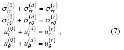
where the superscripts (d) and (r) stand for diffracted and refracted fields, respectively. These conditions have to be enforced for each term, once the solutions have been developed in terms of expansions in spherical coordinates for the diffracted and refracted fields as shown in (5) and (6). Using the expressions in (7) and evaluating in r = a, the system of equations to solve, for each order n is

where An, Dn, En, Fn are the unknown coefficients. y1p(*) (a) , y2p(*) (a) , y3p(*) (a) , y4p(*) (a) are the radial functions at r = a with the same form as that for the incidence of P–waves. These functions have been defined in Appendix A. The superscripts R or E stand for the region where the correspondent function is defined (Figure 1). For region R, spherical Bessel functions are used, while for region E, spherical Hankel functions need to be applied. On the other hand, y1s(*) (a) , y2s(*) (a) , y2s(*) (a) , y3s(*) (a) , y4s(*) (a) are the radial functions at r = a associated to converted S–waves and they are also defined in Appendix A. In the same way as for the P–wave radial functions, these functions have been defined for region R, using Bessel functions while for region E, they are given in terms of Hankel functions. In (µR), and µR are the elastic shear moduli for R and E regions, respectively. Since the boundary conditions for a cavity (ρR = 0) are null tractions acting at the surface of the sphere, the expressions for stress components in (7) must be set to zero. This is achieved by omitting coefficients En and Fn in (8). Thus, the linear system (8) is reduced to two equations.
For the case in which the spherical cavity is filled with fluid (µR= 0), it will be necessary to observe the boundary conditions for pressure and stresses. The equations that govern the fluid are (Mow and Workman, 1966)

where p is the fluid pressure and p = –σrr(t) , In is the unknown coefficient that will be determined when the boundary conditions are satisfied and c = sound velocity of the filler fluid. Then, the boundary conditions for the fluid obstacle at r = a are

with σrθ(t) = 0. In this case, it is necessary to consider the fluid equation in (8). The system will have order three and will be solved exactly.
2.2 S–wave incidence
Let us consider the case in which an elastic S–wave arrives at a spherically symmetric obstacle as shown in Fig. 1. In similar way as it was defined for the P–wave incidence, the total displacement field for an incoming S –wave is given by the superposition principle represented in (1). To construct the S–wave incidence in terms of displacement potentials it will be necessary to calculate

where ø i s the scalar potential and ψ is the vector potential. As we are dealing with a plane S–wave propagating in the positive direction of z–axis and polarized in the positive direction of z– axis, we have
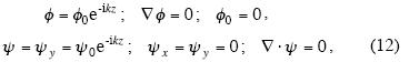
where k=ω/β is the shear wavenumber, ω is the angular frequency, is the S–wave velocity, and i
  is the imaginary unit.
Then, calculating the curl of the vector potential (, we have that the displacement for the x–direction is

with uy(0) = uz(0) = 0 . Doing derivation and considering the incident wave with unitary amplitude, the displacement field for the three directions of movement, written in spherical coordinates, are

Now, it is convenient to write the expressions in (14) as spherical expansions in terms of Bessel and Legendre functions. Einspruch, Witterholt and Truell (1960) displayed most of the basic vector solutions for the incident S–wave displacement field to construct a general expansion in spherical coordinates. However, the definitions of the vector spherical harmonics at the first part of their study have misprints and some inconsistencies in their trigonometric functions, specially into the so–called Hansen vectors L, M, and N. The basic vector solutions for the spherical coordinate system are well given in Morse and Feshbach (1953) and Knopoff (1959b). Thus, the incident field of S–waves can be written as a sum of spherical wave functions, as follows

with

where ur(0) , uθ(0)and uø(0) are the incident fields for the radial, tangential and azimuthal directions, respectively. The radial functions y1s(0) (r) , y3s(0) (r) and y1t(0) (r) are defined in Appendix A. Pn1(cosθ) is the Legendre function of order n and degree m = 1. Since the incident fields are plane waves, only one azimuthal term appears (for P–waves just m = 0 is required, while for SV– or SH–waves, m = 1 is enough). Note that for the incidence of SV– or SH–waves, the azimuthal terms are given by the upper and lower trigonometric functions, respectively. The coefficients Bn and Cn are quite different from those of the P–wave incidence. On the other hand, we have tested the coefficients in (16), verifying them with the plane wave exact solution given by (14) and (13).
To write the part of the incident stress field that contributes to the tractions in the r,θ , and ø directions, we adopt the same formulation as that developed for displacements. Using theBn and Cn coefficients defined above and applying Hooke's law, we are able to write the incident stress field as a sum of spherical wave functions as

where σrr(0) , σrø(0) and σrø(0) are the radial, incident–field stress tensor components (tractions) for the directions r,θ , and ø, respectively. Again, the radial functions y2s(0) (r) , y4s(0) (r) and y2t(0) (r) are defined in Appendix A. Pnx(cosθ) is the Legendre function of order n and degree m = 1. The incidence of SV– or SH–waves is associated to the azimuthal terms (upper and lower, odd or even, trigonometric functions, respectively). There are other components of the stress tensor in spherical coordinates associated to the displacements in (15), but for convenience we omit further mention in this work (the reader is referred to Takeuchi and Saito, 1972, for details). In order to solve a linear system that will be established from boundary conditions, we only require three components of the stress tensor.
To evaluate the corresponding diffracted and total fields, we must expand in spherical wave functions the displacements and stresses for each of these fields. Therefore the incidence is given by a plane S–wave polarized in the positive directions of x– and y– axes as depicted in Figure 1, the produced diffracted fields are of three types, one from the diffraction of P–waves and two from diffracted S–waves. We show in Appendix A the structure of the diffracted and total fields with all participant waves for both displacements and stresses.
Once the forms for refracted and diffracted fields have been established, the unknown coefficients will appear and they need to be determined from the corresponding boundary conditions. The continuity conditions for the stresses and displacements at the elastic sphere interface (r = a) for incident S–waves are given by

where the superscripts (d) and (r) stand for diffracted and refracted fields, respectively.
For instance, if we take a look at the continuity conditions for P–wave incidence, we can find that the components in the ø direction are not present as in this case. Here, we are taking into account the additional terms for displacements and tractions in the latitudinal and azimuthal components. Once the solutions have been developed in terms of the expansions in spherical coordinates for the incident, diffracted and refracted fields, and including the continuity conditions in (18), the system of equations can be constructed. One can recognize that the latitudinal and azimuthal operators will force the coupling terms for the calculation of the unknown coefficients following (18). If we develop and evaluate the solution at r = a, the systems of equations to solve are

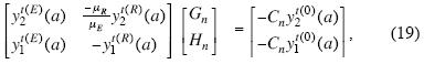
where An , Dn , En , Fn , Gn , and Hn are the unknown coefficients, Bn and Cn are the complex coefficients defined in (16), the radial functions y1s(*)(a) , y2s(*)(a) , y3s(*)(a) , y4s(*) (a) are due to the contribution of all (incident, diffracted and refracted) S–waves, the radial functions y1t(*)(a) , y2t(*)(a) are due to the contribution of toroidal modes. All these groups of radial functions are defined in the Appendix A.
In a similar manner as that for P–wave incidence, the superscripts R or E stand for the region in which the corresponding function is defined (Figure 1). For region R spherical Bessel functions of first kind and order n are used. For region E, spherical Hankel functions must be applied. It is remarkable that only when we deal with the incident field, the radial functions for the region E are Bessel functions. Now the radial functions y1p(*)(a) , y2p(*)(a) , y3p(*)(a), and y4p(*)(a) are aimed to represent converted P–waves.
In (19) µE and µR are shear moduli for E and R regions, respectively. To obtain the spherical cavity case, the boundary conditions are null tractions acting at the surface of the sphere with ρR = 0. The expressions for stress components in (18) must be set to zero. Thus, the linear system is reduced to order two, with a coupling equation that contains the toroidal contribution. This is achieved by omitting coefficients En , Fn , and Hn in (19). For the case in which the spherical cavity is filled with fluid (µR= 0), as for the P–wave incidence case, it is necessary to observe the boundary conditions for pressure and stresses. The appropriate equations that govern the fluid are

where p is the fluid pressure and p = –σrr(t) In is the unknown coefficient that will be determined from boundary conditions, and c = sound velocity of the filler fluid. Note that the azimuthal terms and the Legendre functions are defined with degree m = 1 again, following the azimuthal decomposition for the S–waves. Then, the boundary conditions for the fluid–solid interface at r = a are


with σrθ(t) = 0 . As we are treating with a fluid inclusion, it is
necessary to consider the fluid conditions (20) in the linear system (19). As the equations for the region R in (19) are governed by the shear moduli ratio, these terms must be set to zero. This is equivalent to omit coefficients Dn, En, and Fn. The systems will have again order three for each n.
3. NUMERICAL RESULTS
In order to illustrate some relevant features of the analytic formulations reviewed in previous sections, several computations were performed and relevant results are presented here. Our aim is to provide useful information to calibrate and approximate the seismic response for real objects. The results for a single sphere allow us establishing the basic solutions to construct more complicated formulations, and provide good approximations to observe the scattering behavior for real diffractors in several seismological problems.
Different kinds of materials inside the spherical obstacle, including a cavity, have been analyzed. For example, Figure 2 show the scattering patterns for the diffracted field in the radial direction ur. Calculations for distance r = 2a, with several values of dimensionless frequency ka = 0.25, 0.5, 1.0 and 5.0 are depicted in a figure array. In Figure 2a, the coefficients for the incidence of P–waves and the corresponding partially diffracted P– and S–waves (P–P and P–S, respectively) have been calculated separately. The results correspond to a water–filled sphere (solid line), a cavity (long dashed line) and an elastic sphere with μR / μE = 0.5 (short dashed line). Figure 2b shows the scattering patterns for the incidence of S–waves and the partially diffracted S– and P–waves (S–S and S–P), respectively. In all examples the surrounding medium (matrix) properties are ρE= 2.7 g/cm3, αE = 6.42 x 105 cm/s, βE = 3.04x105cm/s.
The dimensionless frequency η = ka/π (the relationship diameter/wavelength η = 2α/λ, where λ= shear wavelength) allows to establish the various scattering regimes: low–Rayleigh (ka << 1), intermediate–Mie (ka =1) and high–ray (ka >>1). While the first corresponds to large wavelengths and allows for equivalent medium approximations, the last corresponds to ray theory in which relatively simple geometrical descriptions are adequate. Various interesting results emerge from the three models involved by each frame of Figure 2a. First, at low frequencies (ka = 0.25, ka = 0.5) more energy of the incident P–wave field is converted to scattered S–waves than to P–waves, while at intermediate and high frequencies (ka = 1.0, ka = 5.0) the scattered P–wave field is dominant. Second, at low frequencies the amplitudes of the scattered P–waves in the forward and backward directions are comparable, whereas most of the scattered S–wave fields lie in the forward direction. At high frequencies, the amplitudes of the scattered S–waves are several times lower than the scattered P–waves. So, we can accept only generating forward–scattered P–waves. In Figure 2b we observe that at low frequencies (ka = .25, ka = .5) the energy of the incident S–wave field is preserved into scattered S–wave fields. Nevertheless, a considerable amount of scattered energy is converted to P–waves. At high frequencies (ka = 1.0; ka = 5.0) the same effect is identified. At low frequencies, the amplitudes of the scattered S– and P–waves in the forward and backward directions are comparable, whereas at high frequencies, the amplitudes of the scattered S–waves are larger in the forward direction. Note that the amplitude of the scattered S–waves is three to four times larger than the scattered P–waves. In terms of shapes and amplitudes of the scattering diagrams, there are characteristic differences between the fluid–filled, cavity and the proposed elastic models that must be studied with detail in further studies. It is remarkable that the diffracted field distance–dependence behaves very regular, the attenuation effects are geometrical, even stronger than the inverse of distance.
In order to validate our computations we have made several experiments in which elastic, fluid–filled and empty spheres were considered. Various comparisons with some results obtained from the Resonant Scattering Theory (RST) by Gaunard and Uberall (1979a) were performed. Displacement amplitudes for the diffracted fields are computed to show back scattering characteristics. Figures 3 and 4 show the modulus of the rotated diffracted field u (see Appendix B) for P–wave incidence, and ux for S–wave incidence respectively, versus dimensionless frequency η. The receiver is located at x = 0 and z = –7 (r = 7 and θ= π in spherical coordinates) and the matrix properties are the same for both cases (ρE = 2.7 g/cm3, αE = 6.42 ( 105 cm/s, βE = 3.04 x 105 cm/s). From Figure 3 it is remarkable that adding twelve terms (n = 12) to the series of non mode–converted P–wave contribution P–P (top) and mode–converted P–S (bottom) into the diffracted field suffices to produce an accurate graph compared with the reported by RST, on the range 0< η <7. Note that the solid line represents the response of a water–filled sphere with ρR= 1.0 g/cm3, αR = 1.493 x 105 cm/s, the long–dashed line corresponds to an empty sphere (ρR= 0), and the short–dashed line to an elastic sphere with properties μR / μE= 0.5. The P–S coefficients are offered in the same range of frequencies as for P–P case. The similarity of spectral characteristics for both P–P and P–S plots is remarkable (mode–excitation, periodicity and amplitudes). For example, the periodicity effect is preserved on both plots and mainly in the fluid case. We must note that the energy is well concentrated in recursive patterns of spectral spikes (resonant modes, adopting the engineering term). Although the observation point is located over a nodal axis the behavior of the given frequency responses are representative of all locations.
In Figure 4 same kind of results were computed for the incidence of a S V–wave. Corresponding coefficients S–S and S–P were calculated in order to study the spectral characteristics of the response. Twelve terms were used (n = 12) to compute non mode–converted partial S–wave contributions S–S (top) and mode–converted S–P (bottom) of the diffracted field. Again, the solid line represents the water–filled sphere, the long dashed line corresponds to an empty sphere and the short dashed line to an elastic sphere with properties given by μR / μE= 0.5. Remarkably, the fluid response for the S–S coefficients is very strong and rippled for all frequencies, as compared with those of the cavity and elastic cases. The S–P coefficients show the same excited modes and weak amplitude rapidly attenuated with respect to frequency. Unfortunately, RST does not consider the case of an incoming S–wave. Similar results on this matter are due to Korneev and Johnson (1996) for some deterministic models. Now it is possible with these results to establish a comparison for the back–scattered field between non mode–converted and mode–converted S–waves. Even though the spectral plots are completely different from those of the P–wave calculations, the same resonances are excited by an incident shear wave as by an incident compressional wave.
In order to observe the propagation features and to continue with the study of incident elastic P– and S–waves over an empty, fluid–filled and elastic sphere, various configurations for geophysical applications have been experimented in time domain. A three–dimensional behavior is offered with the aim to give a better understanding of the time–space complexity in the models. Synthetic seismograms are helpful to observe and understand diffraction effects and polarization patterns. Traces were obtained by convolution with a Ricker wavelet followed by an inverse Fourier transform. In the synthetic seismograms presented here a Ricker wavelet with characteristic frequency ωc=1/π, tp = 1s and t s=5s is used for all examples.
Figure 5 shows synthetic seismograms for two components of displacement (Ux and Uz). We omit the displacement along the y–axis, Uy, for both incidences because Uy = 0. For the SH–wave incidence the results (not shown here) are identical due to symmetry. Figure 5a depicts the P–wave incidence upon an elastic ρR/ρE=1.0, μR / μE=0.5) (top), cavity (middle) and water–filled (bottom) sphere plotted versus time. Matrix properties are ρE= 2.7 g/cm3, αE = 6.42 x 105 cm/s, βE = 3.04 x 105 cm/s. To observe the propagation and diffraction effects after the interaction between the incoming wave and the spherical obstacle, there are 51 receivers at x = ±3a and z = 2a, as illustrated in configuration (A–A') of Figure 1. In the elastic case, it is possible to observe a strong and delayed amplification of the incident field at Uz, due to the soft properties of the sphere. Normal P–wave incidence clearly shows how the incident field is delayed by the presence of an empty sphere at the Uz component. The diffracted field across the cavity model is the result of scattered waves generated at the surface of the sphere, see both Ux and Uz. The traces for the water–filled sphere again show that the diffracted field is mainly composed of waves scattered by the cavity and the appearing of resonant fluid P–waves at 8s.
In order to simulate a typical array of seismometers on surface, Figure 5b shows synthetic seismograms for two components of displacement Ux and Uz over the section B–B' illustrated in Figure 1. In this result, the time response of a plane P–wave that arrives over an elastic (top), cavity (middle), and water–filled (bottom) sphere, is depicted. The matrix properties are the same as the previous examples. Along the three cases the direct wave is easily seen. Note that the diffracted wave in the elastic sphere appears with a very strong attenuation over the first half of receivers. Again a set of propagating fluid–generated waves appears at 8.5s. The diffracted wave appears clearly for the cavity and the water–filled sphere.
Figure 5c shows synthetic seismograms for two components of displacement Ux and Uz in the same configuration of Figure 5a. In this set of results, the time response of an incident S V–wave over an elastic (top), cavity (middle), and water–filled (bottom) sphere is illustrated. The SV–wave incident field appears to be delayed for the three kinds of inclusions. In the elastic case, a large amplification occurs and a strong scattered wave is generated. The cavity and elastic cases are very similar, if the amplification effect by the soft material of the elastic sphere is neglected. In the water–filled case a considerable attenuation effect at the central receivers is observed, this is due to the presence of the fluid. We must note that a strong train of fluid field generated P–waves propagating around 7s in both components of movement is clearly appreciated.
Finally the Figure 5d shows synthetic seismograms for two components of displacement Ux and Uz over the section B–B'. The seismic response of an incident SV–wave over an elastic (top), cavity (middle), and water–filled (bottom) sphere is displayed. The same properties as those for Figure 5b were adopted. The difference between the elastic and cavity responses generated by the diffracted wave is not so clear in comparison with those of 5b plot. This may be explained due to the polarization of the incident field and the position of receivers. However, some diffracted waves can be followed from the Uz component for the three kinds of inclusions. If we look at the cavity and the fluid–filled sphere seismograms, we can recognize two sets of trains of P–waves generated by the diffraction of the incident field with the edges of the sphere at 4s and 8s. However a strong reflection of a P–wave generated by the fluid is observable at 10s. It has been seen clearly that the fluid effect and resonance on the S–wave propagation it is detectable.
4. CONCLUSIONS
We have presented a review of the analytic solution for the scattering of P– and S–waves by a single spherical obstacle. The expansions of plane P– and S–waves in terms of spherical Bessel functions and Legendre polynomials using the relations for the displacements and stresses were re–derived. We give a complete and revised table of such coefficients. In order to obtain an accurate approximation of the harmonic wave solution, we identified that the order of the series expansions n must be at least the maximum number of dimensionless frequency in the calculation (according to Takeuchi and Saito, 1972). We believe that a reasonable rule of thumb is then n = max(ka). Results from elastic, fluid–filled and empty spheres were analyzed in frequency domain. We performed some calculations in which the radial diffracted field was computed for low–Rayleigh (ka <<1), intermediate–Mie (ka = 1) and high–ray (ka >> 1) scattering regimes. A number of interesting observations were discussed from the calculations of P– and S–waves scattering patterns. We performed several computations comparing with some results obtained from the well–known Resonant Scattering Theory (RST) by Gaunard and Uberall (1979a). Diagrams for the displacement amplitudes for the diffracted field showing back scattering characteristics were computed. In the cases of fluid–filled sphere and cavity, the comparisons versus RST show spectral plots very accurate to those sketched here. From our results it is possible to observe that it is extremely necessary to compute series of multiple examples in 3D to establish a complete data set and robust characterization of the phenomenon. In order to study the propagation features, various configurations of seismological interest were computed in time domain. To observe scattering and diffraction and to simulate standard arrays of seismometers located on the surface, two configurations of receivers were analyzed (A–A' and B–B'). Such analyses allow us to establish approximate seismic responses for smooth objects or buried real structures that might be modeled as spheres.
Results presented in this paper should also be applicable, in at least an approximate manner, to geophysical and engineering problems involving scattering from heterogeneities more complicated than a simple sphere. Scattering by a sphere serves as a canonical problem for a general class of objects with relatively simple and smooth boundaries. The main multiple scattering methods commonly neglect the high–frequency terms of the basic solutions in 2– and 3–D. Generally, they adopt low contrast in the model's properties ratio or low frequency approximations. In spite of this, we believe that the analytic solutions offer a trustworthy path to compute the scattering and seismic response by single or multiple heterogeneities. Constructing more complicated formulations or approximate solutions aimed to understand real problems should start with this classical solution.
5. ACKNOWLEDGEMENTS
Thanks are given to Federico J. Sabina–Císcar and Carlos Valdés–González for their assistance and invaluable discussion on the formulation presented here. We also thank S. K. Singh, V. Levin, S. Chávez–Pérez and G. Quiroga–Goode, for their comments and suggestions to improve this work. This research was partially supported by CONACYT project NC–204 and by Instituto Mexicano del Petróleo, Gerencia de Prospección Geofísica and Naturally Fractured Reservoirs Program under grant YNF–D1341.

6. Bibliography
ABRAMOWITZ, M. and I. A. STEGUN, 1964. Handbook of mathematical functions with formulas, graphs and mathematical tables, National Bureau of Standards, Applied Mathematics series 55. [ Links ]
AKI, K. and P. G. RICHARDS, 1980. Quantitative seismology, Theory and methods, W. H. Freeman and Co., San Francisco. [ Links ]
BOSTROM, A. and A. ERIKSSON, 1993. Scattering by two penny–shaped cracks with spring boundary conditions, Proc. R. Soc. Lond., 443,183–201. [ Links ]
BOUWKAMP, C. J., 1954. Diffraction theory, Repts. Prog. Physics., 17, 35–100. [ Links ]
CHAPMAN, C. H. and R. A. PHINNEY, 1970. Diffraction of P waves by the core and an inhomogeneous mantle. Geophys. J. R. Astr. Soc., 21, 185–205. [ Links ]
CORMIER, V. F. and P. G. RICHARDS, 1977. Full wave theory applied to a discontinuous velocity increase: The inner core boundary. J. Geophys., 43, 3–31. [ Links ]
EINSPRUCH, N. G., E. J. WITTTERHOLT and R. TRUELL, 1960. Scattering of a plane transverse wave by a spherical obstacle in an elastic medium. J. Appl. Phys., 31, 806–818. [ Links ]
ERINGEN A. C. and E. S. SUHUBI, 1975. Elastodynamics, Academic Press, New York. [ Links ]
FUNG, Y. C., 1965. Foundations of solid mechanics, Prentice–Hall Inc., Englewood Cliffs, N.J. [ Links ]
GAUNARD, G. C. and H. UBERALL, 1979(a). Numerical evaluation of modal resonances in the echoes of compressional waves scattered from fluid–filled spherical cavities in solids. J. Appl. Phys., 50, 4642–4660. [ Links ]
GAUNARD, G. C. and H. UBERALL, 1979(b). Deciphering the scattering code contained in the resonance echoes from fluid–filled cavities in solids. Science, 206, 61–64. [ Links ]
GAUNARD, G. C. and H. UBERALL, 1980. Identification of cavity fillers in elastic solids using the resonance scattering theory, Ultrasonics., 261–269. [ Links ]
GRITTO, R., V. A. KORNEEV and L. R. JOHNSON, 1995. Low frequency elastic wave scattering by an inclusion: Limits of applications. Geophys. J. Int., 120, 677–692. [ Links ]
GRITTO, R., V. A. KORNEEV and L. R. JOHNSON, 1999. Nonlinear three–dimensional inversion of low frequency scattered elastic waves. Pure Appl. Geophys., 156, 557–589. [ Links ]
KNOPOFF, L., 1959(a). Scattering of compression waves by spherical obstacles. Geophys., 24, 30–39. [ Links ]
KNOPOFF, L., 1959(b). Scattering of shear waves by spherical obstacles. Geophys., 24, 209–219. [ Links ]
KORNEEV, V. A. and L. R. JOHNSON, 1993(a). Scattering of elastic waves by a spherical inclusion–I. Theory and numerical results. Geophys. J. Int., 115, 230–250. [ Links ]
KORNEEV, V. A. and L. R. JOHNSON, 1993(b). Scattering of elastic waves by a spherical inclusion–II. Limitations of asymptotic solutions. Geophys. J. Int., 115, 251–263. [ Links ]
KORNEEV, V. A. and L. R. JOHNSON, 1996. Scattering of P and S waves by a spherically symmetric inclusion. Pure Appl. Geophys., 147, 675–718. [ Links ]
McMECHAN, G. A., 1982. Resonant scattering by fluid–filled cavities. Bull. Seism. Soc. Am., 72, 1143–1153. [ Links ]
MONTALTO, A., V. LOGO and G. PATANE, 1995. Echo–resonance and hydraulic perturbations in magma cavities – application to the volcanic tremor of the Etna (Italy) in relation to its eruptive activity. Bull. Vulcanol, 4, 219–228. [ Links ]
MOROCHNIK, V. S., 1983(a). Scattering of shear elastic waves by a low–contrast spherical inclusion, Izvestia Acad. Nauk USSR. Fizika Zemil, 6,41–49. (in Russian) [ Links ]
MOROCHNIK, V. S., 1983(b). Scattering of compressional elastic waves by a low–contrast spherical inclusion, Izvestia Acad. Nauk USSR. Fizika Zemil 7, 65–72. (in Russian) [ Links ]
MORSE, P. M. and H. FESHBACH, 1953. Methods of theoretical physics, McGraw–Hill, New York. [ Links ]
MOW, C.C., 1965. Transient response of a rigid spherical inclusion in an elastic medium. J. Appl. Mech., 32, 637–642. [ Links ]
MOW, C. C. and Y. H. PAO, 1971. The diffraction of elastic waves and dynamic stress concentrations, A report prepared for United States Air Force Project Rand. [ Links ]
MOW, C. C. and J. W. WORKMAN, 1966. Dynamic stresses around a fluid–filled cavity. J. Appl. Mech., 793–799. [ Links ]
PAO, Y. H. and C. C. MOW, 1963. Scattering of a Plane Compressional Wave by a Spherical Obstacle. J. Appl. Phys., 34, 493. [ Links ]
PAO, Y. H. and C. C. MOW, 1973. The diffraction of elastic waves and dynamic stress concentrations. Crane and Russak, New York. [ Links ]
RAYLEIGH, LORD, 1872. Investigation of the disturbance produced by a spherical obstacle on the waves of sound, Proc. London Math. Soc., 4, 253–283. [ Links ]
TAKEUCHI, H., 1950. Diffraction of elastic waves by an elastic sphere. Geophys. notes, 3, 1–28 [ Links ]
TAKEUCHI, H. and M. SAITO, 1972. Seismic surface waves, Methods in computational physics, 1, II, B. A. Bolt, ed., Academic Press, New York and London. [ Links ]
VEKSLER, N. D., J. L. IZBICKI and J. M. CONOIR, 1999(a). Elastic wave scattering by a cylindrical shell. Wave motion, 3, 195–209. [ Links ]
VEKSLER, N. D., J. L. IZBICKI and J. M. CONOIR, 1999(b). Flexural waves in the acoustic wave scattering by a liquid–filled shell. Acoust. Phys., 3, 279–288. [ Links ]
VEKSLER, N. D., A. LAVIE and B. DUBUS, 2000. Peripheral waves generated in a cylindrical shellwith hemispherical endcaps by a plane acoustic wave at axial incidence. Wave motion, 4, 349–369. [ Links ]
WOLF, A., 1945. Motion of a rigid sphere in an acoustic wave field. Geophys., 10, 91. [ Links ]
WU, R. and K. AKI, 1985. Scattering characteristics of elastic waves by an elastic heterogeneity. Geophys., 50, 582–595. [ Links ]
YING, C. F. and R. TRUELL, 1956. Scattering of a plane longitudinal wave by a spherical obstacle in an isotropically elastic solid. J. Appl. Phys., 27, 1086–1097 [ Links ]

