


 texto en
  Inglés (pdf)
 Artículo en XML
 Referencias del artículo
 Enviar artículo por email
 Citado por SciELO
  Similares en
SciELO
Similares en
SciELO 
 Permalink
Introduction
Among the services provided by a basin, environmental services, including hydrological ones whose quantity and quality characteristics depend on the climate and conservation conditions under which it is located, are of particular importance (Duque-Yaguache & Vázquez-Zambrano, 2015). The ability of a basin to provide hydrological services depends on interlocking features that are heterogeneously distributed in its area (Isik, Kalin, Schoonover, Srivastava, & Lockaby, 2013), which are: topography, plant cover, land use and climate (Brauman, Daily, Duarte, & Mooney, 2007).
In many arid regions, water scarcity is a topic of interest that prompts hydrological research focused on the aspects that characterize them (Loyer, Estrada, Jasso, & Moreno, 1993). In these studies, whether of a basin or ecosystem, an important topic is the simulation of processes, in which the user can obtain data related to the behavior of a system through a model whose cause and effect relationship is the same as (or similar to) that of the original system (Sánchez-Cohen, 2005).
At basin level, hydrological modeling is an indispensable component of water resources research and management (Johnston & Smakhtin, 2014). At present, there are several computational tools for modeling hydrological processes, each one defined by the type of parameters used as input and its specific field of application.
Among the most used models are: a) MODFLOW, used to simulate groundwater systems in confined and unconfined aquifers, and also considers recharge flows, evapotranspiration, extractions, rivers and drains (Chen, Izady, & Abdalla, 2017); b) the Soil & Water Assessment Tool (SWAT), which allows simulating the effects on hydrological variables as a result of management practices carried out in basins (Dunea et al., 2016); c) the Hydrological Bureau Water balance-section (HBV) was developed by the Swedish Hydrological and Meteorological Institute in 1976 and has been applied under various climatic conditions and scales (Güitrón, 2007), and d) the Water Evaluation and Planning System (WEAP), which is used for the planning and distribution of water resources and can be applied to different scales (Adgolign, Srinivasa-Rao, & Abbulu, 2016). WEAP includes water demands with associated priorities and uses scenarios to assess the impacts and different water resource distribution schemes in the basin (Amisigo, McCluskey, & Swanson, 2015; Johannsen, Hengst, Goll, Höllermann, & Diekkruger, 2016).
According to Lalika, Meire, Ngaga, and Chang’a, (2014), watersheds and their rivers are ecologically vital for the health, welfare and prosperity of human beings; however, anthropogenic activities, coupled with climate variability and change, are degrading them. These events are presented as one of the major concerns due to the possible effects of climate change on water resources (Martínez-Austria, & Patiño-Gómez, 2012). In addition, the pressure on water resources is increasingly aggravating their availability, especially in areas with low rainfall.
In Mexico, a basin that includes the Sextín or Oro (Gold) River is located in the Sierra Madre Occidental. From its source to its confluence with the Ramos River, in the reservoir of the Lázaro Cárdenas (El Palmito) dam, it covers an 8,248 km2 area, extends 245 km in length (Secretaría de Recursos Hidráulicos [SRH], 1970) and has an average annual surface water availability, up to the Sardinhas hydrometric station, of 102.7 Mm3 (Diario Oficial de la Federación [DOF], 2016). In 1970, operations began at the Sardinas station, located on the Sextín River, 390 m upstream from the confluence with the Sardinas stream, 1 km west of the village of the same name and 12 km northwest of the town of San Bernardo, situated within the municipality of the same name in the state of Durango, Mexico (Comisión Nacional del Agua [CONAGUA], 2016b). This station was created with the objective of determining the hydraulic regime of the stream, as well as its contributions to the Lázaro Cárdenas dam (CONAGUA, 2016a; SRH, 1970).
The aim of this study was to evaluate the impact of variations in climate patterns on runoff from the Sextín River basin through the WEAP model in order to have analytical and support tools in decision making where there is climate uncertainty.
Materials and methods
Study area
This study was carried out in the upper part of the Nazas River, belonging to Nazas-Aguanaval hydrological region No. 36 located in the central-northeast of Durango, Mexico (Figure 1). The study basin covers a 5,019.88 km2 area and is part of the Sierra Madre Occidental. Its annual precipitation ranges from 480 to 650 mm, the average annual maximum and minimum temperatures are 25.8 and 1.9 °C, respectively (Instituto Mexicano de Tecnología del Agua [IMTA], 2009), and its average annual volume of natural runoff is 523.56 Mm3 (CONAGUA, 2016a). The basin covers part of the municipalities of Tepehuanes, Guanaceví, Ocampo, San Bernardo, Indé and El Oro, Durango, Mexico.

Delimitation of the basin
The processes for developing the hydrological scheme in WEAP involve delimitating the basin, and if possible delimitating it to sub-basins. For this, we used the vector information from the watershed water flow simulator (SIATL for its initials in Spanish), which classifies the study area into five sub-basins (Table 1; Instituto Nacional de Estadística y Geografía [INEGI], 2016).
Table 1 General characteristics of the sub-basins considered in the study.
| Sub-basin | Key | Perimeter (km) | Area (km2 ) | Max. elevation (m) | Min. elevation (m) | Mean slope (%) |
|---|---|---|---|---|---|---|
| El Oro | RH36Cg | 276.95 | 2445.27 | 3140 | 1800 | 28.49 |
| San Esteban | RH36Cf | 177.59 | 716.54 | 3140 | 1800 | 37.83 |
| De Lobos | RH36Ce | 166.91 | 515.11 | 3260 | 1700 | 37.91 |
| Matalotes | RH36Cd | 186.84 | 891.90 | 2980 | 1660 | 34.82 |
| Sextín | RH36Cc | 216.29 | 451.06 | 2700 | 1639 | 29.48 |
The altitudinal gradient in the study area ranges between 1,600 and 3,260 m, with an average slope of 33 %. Specifically, for the Sextín sub-basin, an autonomous delimitation was made, because the gauging station was in an intermediate zone and the total area did not represent the actual runoff in the study area (Figure 2). The hydrometric station used for delimitating the basin corresponds to the Sardinas station (key 36071), located in the municipality of San Bernardo at 1,639 masl (26° 5’ 3’’ North latitude and 105° 33’ 57’’ West longitude; CONAGUA, 2016b).

Climatological and hydrometric information
For the hydrological model, historical temperature, relative humidity, wind speed and cloud cover time series were used, all on a monthly scale. Two climatological information sources were used: stations operated by the National Meteorological Service (SMN for its initials in Spanish) and the network of automated stations run by the Instituto Nacional de Investigaciones Forestales, Agrícolas y Pecuarias (INIFAP, 2016). From the first source, an analysis was made of the consistency and homogeneity of the information contained at 11 weather stations present inside and outside the study area; of the 11 stations four were used. Regarding the second source, only one weather station was used: Puerta de cabrera (Table 2; IMTA, 2009). It should be pointed out that the above-mentioned station was only used to parameterize the WEAP hydrological model; however, it was not considered in the generation of climate scenarios due to its short data period.
Table 2 Weather stations considered in the study.
| Weather station | Latitude | Longitude | Elevation | First datum | Last datum |
|---|---|---|---|---|---|
| Cendradillas | 26° 16’ 58’’ | 106° 00’ 38’’ | 2,500 | 01/1961 | 01/2008 |
| Ciénega de Escobar | 25° 36’ 03’’ | 105° 44’ 47’’ | 2,144 | 04/1965 | 01/2009 |
| Guanaceví | 25° 55’ 59’’ | 105° 57’ 06’’ | 2,300 | 06/1922 | 01/2009 |
| Sardinas | 26° 05’ 03’’ | 105° 33’ 56’’ | 1,639 | 05/1970 | 05/2009 |
| Puerta de cabrera | 26° 03’ 26.9’’ | 105° 15’ 19.3’’ | 1,911 | 06/2006 | 01/2017 |
Data missing from the stations were calculated with a climate generator (Esquivel, Cerano, Sánchez, López, & Gutiérrez, 2015); from these stations, temperature and precipitation information was used. The variables relative humidity and wind speed were acquired from the automated Puerta de Cabrera station located in the municipality of Indé and belonging to the INIFAP network of weather stations (INIFAP, 2016). The cloud cover fraction percentages were inputted empirically. The hydrometric information inputted into the model corresponds to Sardinas station 36071, from 1971 to 2004, obtained from the National Surface Water Databank (BANDAS; CONAGUA, 2016b).
Land use and vegetation
The parameterization of land use and vegetation (cover) present in each sub-basin was done with INEGI's Series III 1:250,000 scale. From the above, it was determined that the study basin is composed of coniferous forest (47.6 %), oak forest (26 %), grassland (16.9 %), induced vegetation (4.7 %), agricultural-livestock-forestry use (ALFU, 4.5 %) and bare ground (0.3 %). The WEAP model does not require inputting specific soil parameter data (e.g. physical properties), but it does need: crop coefficient (Kc), water storage capacity in the root zone (Sw), water storage capacity in the deep zone (Dw), runoff resistance factor (RRF), root zone conductivity (Ks), deep zone conductivity (Kd), preferential flow direction (f), initial moisture level in root zone (Z1) and initial moisture level in deep zone (Z2). These values were inputted as a percentage or absolute number. The adjustments made in these variables are carried out considering the ranges established by the same model and other hydrological schemes similar to the study basin (Flores-López, Galaitsi, Escobar, & Pukey, 2016).
Description and parameterization of WEAP
WEAP allows users to create specific models, which can calculate hydrological changes by considering alterations caused by environmental conditions or infrastructure (Flores-López et al., 2016).
Yates, Sieber, Purkey, Hubber-Lee, and Galbraith (2005a , 2005b) and Yates et al. (2007) describe WEAP as a continuous model configured as a set of contiguous sub-basins covering the entire extent of the basin under study. A homogeneous set of climatic data (precipitation, temperature, relative humidity and wind speed) is used in each sub-basin, which are divided into different types of land cover/use (Centro de Cambio Global [CCG], 2009).
Within the system, a quasi-physical one-dimensional model, with two water balance buckets for each type of land cover/use, distributes water among surface runoff, infiltration, evaporation, base flow and percolation. Data from each area are summed to obtain the aggregate values in a sub-basin. At each model run time, WEAP first calculates the hydrological flows, which are transferred to the associated rivers and aquifers (Figure 3). For the calculation of evapotranspiration, the model intrinsically uses the Penman-Monteith equation (Sieber & Purkey, 2015).
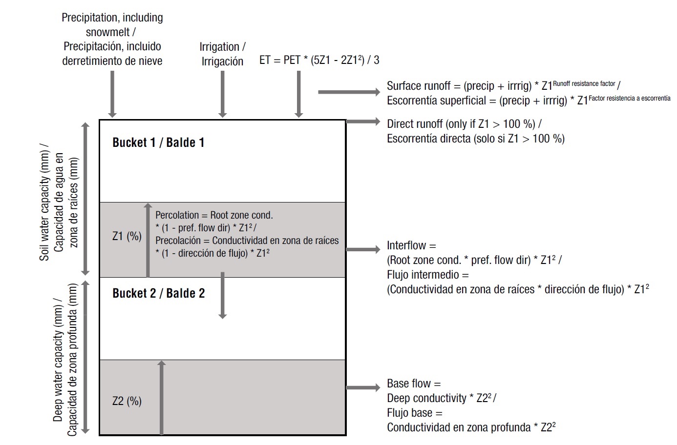
Figure 3 Hydrological elements modeled in WEAP (Centro de Cambio Global [CCG], 2009). §ET: evapotranspiration, PET: potential evapotranspiration, Z1: initial moisture level in root zone, Z2: initial moisture level in deep zone
WEAP requires inputting of climatological and plant cover data to estimate the components of the hydrological balance for each basic spatial hydrological unit that has to be identified in the model. These basic units correspond to catchment areas, named in the model as catchments (CCG, 2009).
The resolution of the catchments in WEAP can be adjusted based on the density of available weather stations. In regions with scarce information, the number of hydrological units may be smaller; however, it allows preserving the representativity of the basin as a whole (Flores-López et al., 2016).
The climatic data required to perform the modeling are precipitation, temperature, humidity, wind, melting point, freezing point, latitude, and initial amount of snow (in the event this variable is relevant, CCG, 2009). In addition, flow data are needed at measuring stations in order to be able to compare the results of the model and perform calibrations.
Model calibration
Quantification of the differences between observed and generated data helps to estimate the degree of reliability of the model results. Changing certain conditions in the system allows adjusting the model values to the actual values. In this case, the variables that were changed in the model and that showed sensitivity in the results were: runoff resistance factor (RRF), preferential flow direction (f), initial moisture level in the root zone (Z1) and initial moisture level in the deep zone (Z2). The adjustments carried out in these variables were made considering the ranges established by the model and by other hydrological schemes similar to the study basin (Flores-López et al., 2016).
In this study, the model was not validated since the research objective was to find the best predictive efficiency of the model based on observed runoff, but not to make projections. Land use and vegetation were used so that the measured runoff data represent, as closely as possible, the plant cover that existed at the time. Nevertheless, to measure the model’s predictive efficiency we used some indicators frequently used in hydrological modeling (Ahmed, 2012), which are listed below:
Percentage BIAS (% BIAS)
This indicator can be thought of as the average of residuals as a fraction of the average flow (Equation 1). It is also equivalent to the cumulative flow volume error relative to observed volume, which is usually known as water balance error in the hydrologic modeling literature. In general, lower values of % BIAS indicate better model efficiency.
 (1)
(1)
Regression coefficient (R2)
It expresses the strength of association between two variables. R 2 = 1 indicates a perfect positive relationship between two variables, but is not an automatic guarantor of good simulation as it is insensitive to additive and proportional differences between observed and predicted time.
 (2)
(2)
Nash-Sutcliffe coefficient of efficiency (NSE)
This coefficient has been widely used by hydrologic modelers. NSE can be thought of as the ratio of the mean square error to the variance of observed data, subtracted from unity. The value of NSE varies from - ∞ to 1, with 1 being the optimal value. Generally, values between 0 and 1 are deemed acceptable, whereas values < 0 indicate that the mean observed value is a better predictor of simulated values, implying that the model's efficiency is unacceptable.
 (3)
(3)
Climate change scenarios
To obtain future regionalized climate change scenarios, the LARS-WG v4.0 climate generator was used. This stochastic generator creates daily time data for a particular site with the same statistical characteristics as the station's actual series (Camargo-Bravo & García-Cueto, 2012).
The climate scenarios used were created by Regionalized Climate Models for Mexico (MCRM for its initials in Spanish), developed by UNAM’s Atmospheric Sciences Center, and contemplate time horizons denoted as 2020s and 2050s, which comprise 30-year averages (2010-2039 for 2020s, 2040-2069 for 2050s; Conde-Álvarez & Gay-García, 2008). For this study, future synthetic series were created for the A2 and A1B climate change scenarios, established by the Intergovernmental Panel on Climate Change (IPCC), for the years 2020s and 2050s. The former is characterized by a continuously increasing population, but with lower economic growth than in other scenarios; it also maintains a high increase in greenhouse gas emissions. The latter describes a world with rapid economic growth, reaching its maximum population in the middle of this century; it adopts more efficient technologies and takes a balanced approach to the use of energy sources.
Results and discussion
In Mexico, several studies on hydrological systems have been carried out based on the WEAP simulation program. These include the Guayalejo-Tamesí River basin in Tamaulipas, Mexico, which consisted of modeling the effects of climate change on the availability of water for domestic, industrial and agricultural use. The results showed a greater vulnerability on the part of the agricultural sector to climate change for the A2 and B2 emission scenarios (Sánchez-Torres, Ospina-Noreña, Gay-García, & Conde, 2009), the latter less adverse to meet the region's water demand. Another application in Mexico with WEAP was in the Rio Grande/Bravo basin (Sandoval-Solís & McKinney, 2009); however, there is little development of public policies in relation to the management of water resource in Mexico.
For the basin under study, Figure 4 shows the data observed and simulated by the model. It can be observed that the global simulation in the calibration period (1971-2004) is acceptable and indicates the ability of the model to predict, in general, the hydrological response of the basin.

The flow duration curve is representative of the current’s average flow regime, so it can be used to predict the behavior of the future regime in the basin analyzed (Figure 5).

The NSE value was 0.81 and the % BIAS 12.1, considered very good and satisfactory, respectively (Moriasi et al., 2007), while R2 was 0.81.
Regarding the future climate change scenarios obtained for both the maximum (Tmax) and minimum (Tmin) temperature, in the four stations analyzed, increases of 0.6 to 1.3 °C and 0.7 to 1.6 °C respectively were projected. The above takes into account both scenarios analyzed in the 2020s. With regard to rainfall (Rf), the results indicated an increase of 30 to 70 mm on average for stations located in the basin, except for Guanacevi, which showed decreases (3 %) relative to the historical average (Table 3).
Table 3 Weather stations analyzed in the projected period (2020s).
| Variable | Scenario | Weather stations | |||
|---|---|---|---|---|---|
| Cendradillas | Ciénega de escobar | Guanaceví | Sardinas | ||
| Tmax* (°C) | Historical | 21.5 | 22.9 | 23.2 | 25.8 |
| A1B | 22.8 | 23.6 | 24.3 | 26.6 | |
| A2 | 22.7 | 23.5 | 24.3 | 26.6 | |
| Tmin (°C) | Historical | 1.9 | 6.4 | 7.2 | 6.3 |
| A1B | 3.5 | 7.1 | 8.0 | 7.4 | |
| A2 | 3.5 | 7.1 | 8.0 | 7.4 | |
| Rf (mm) | Historical | 585 | 580 | 650 | 486 |
| A1B | 618 | 607 | 647 | 555 | |
| A2 | 605 | 594 | 634 | 549 | |
*Tmax: maximum temperature, Tmin: minimum temperature, Rf: rainfall, A1B: scenario with rapid economic growth, A2: scenario with continuously increasing population.
For the second projected period (2050s), Tmax presented an increase from 1.5 to 2.1 °C and Tmin from 1.5 to 2.4 °C, considering the A2 and A1B scenarios. The Rf results showed an increase of 12 to 60 mm on average for the basin stations, except for Guanacevi, which showed decreases (2.8 %) in its average value compared to the historical one (Table 4).
Table 4 Weather stations analyzed in the projected period (2050s).
| Variable | Scenario | Weather stations | |||
|---|---|---|---|---|---|
| Cendradillas | Ciénega de escobar | Guanaceví | Sardinas | ||
| Tmax* (°C) | Historical | 21.5 | 22.9 | 23.2 | 25.8 |
| A1B | 23.6 | 24.4 | 25.2 | 27.5 | |
| A2 | 23.6 | 24.4 | 25.2 | 27.4 | |
| Tmin (°C) | Historical | 1.9 | 6.4 | 7.2 | 6.3 |
| A1B | 4.3 | 7.9 | 8.8 | 8.2 | |
| A2 | 4.3 | 7.9 | 8.8 | 8.2 | |
| Rf (mm) | Historical | 585 | 580 | 650 | 486 |
| A1B | 610 | 599 | 640 | 546 | |
| A2 | 599 | 592 | 632 | 546 | |
*Tmax: maximum temperature, Tmin: minimum temperature, Rf: rainfall, A1B: scenario with rapid economic growth, A2: scenario with continuously increasing population.
It should be pointed out that Tmax, Tmin and Rf maintain a similar behavior in both periods and scenarios analyzed. However, the annual Tmin shows a broader range than the annual Tmax between observed and generated values, for both the 2020s and the 2050s, which may suggest that the thermal amplitude has decreases in general. In terms of climate change, it should be considered that temperature oscillations can positively or negatively impact various systems and processes (Landa, Magaña, & Neri, 2008).
Also, the magnitude of the projected increases in temperature increases the longer the term and between greenhouse gas emission (GHG) scenarios; the higher the emissions considered, the higher the temperature increase (Secretaría de Medio Ambiente y Recursos Naturales - Instituto Nacional de Ecología [SEMARNAT-INE], 2009). Regarding annual cumulative Rf, the assemblage of projections indicates that the rains will decrease in much of the country towards the middle and end of this century (SEMARNAT-INE, 2009).
The dispersion between experiments is very wide, reflecting the great uncertainty in rain projections. Contrary to what was reported by SEMARNAT-INE (2009), the results showed increases in 75 % of the analyzed stations. On the other hand, to assess the impact of climate scenarios on the basin’s water balance, the climate part within the hydrological scheme was replaced by the data series generated by LARS-WG for each station, while the other model parameters remained constant (Figure 6).

The A1B scenario, in the 2020s period, projected a 9.6 % increase in the basin’s mean annual flow, while for A2 it was 3 %. The above is an effect of the possible increase in rainfall in the stations analyzed. In the second period analyzed (2050s), the A1B scenario showed a 4.2 % increase in mean annual flow; however, the A2 scenario reflected a decrease of 3.3 %, considering the precipitation levels obtained by the climate generator. The average historical value observed for basin runoff was 523.5 Mm3, so that, in general terms, assuming an increase in Rf, the model predicted increased runoff for both scenarios.
Conclusions
The projections of the regionalized climate change scenarios predicted an increase in the three variables analyzed for the majority of the basin’s weather stations (minimum temperature, maximum temperature and precipitation). An increase of 1 °C is anticipated due to the potential impacts that could have repercussions in terms of crop water requirements, forest species, etc.
The increase in precipitation is not necessarily considered a good condition, taking into account the temporality in which it could occur. Likewise, an increase in runoff is projected for the two periods analyzed (2020s and 2050s); however, subsequent analyses need to assess the impact it might have on processes such as erosion. Further studies are recommended with other climate models that allow making comparisons and determining trends in order to have a better understanding and analysis of future risks due to climate change.

