


 nueva página del texto (beta)
 Inglés (pdf)
 Artículo en XML
 Referencias del artículo
 Enviar artículo por email
 Citado por SciELO
  Similares en
SciELO
Similares en
SciELO 
 Permalink
1. Introduction
The growth of machine learning and Deep learning (DL) exponentially introduced significant modifications in different fields and implementations by emerging algorithms, which draw inspiration from a wide range of domains including alpine skiing, Coronavirus mask protection, and gravitational search strategies. Image processing is utilized in materials science, aerospace, photogrammetry, particle physics, geology, and medicine, among other disciplines. Frequently, preparatory stages are executed in the domain of the image processing before localization including the implementation of sophisticated DL methods to improve the precision of diagnoses or extract crucial attributes (Ahmed et al., 2024) . Image denoising is an essential operation, as it eliminates noise to produce flawless photographs while maintaining their intrinsic qualities. The consistent problem arises from the existence of several types of noise, including Poisson noise, salt and pepper noise, Gaussian noise, and speckle noise. This recurring issue frequently arises because of deficiencies in the sensors used in the camera or during the procedures o transmitting images (Gonzalez & Woods, 2008) .
In image processing, Convolutional Neural Networks (CNNs) have gained popularity because their performance is superior to that of prior techniques. One of the many capabilities of CNNs is data preparation and processing. They have improved algorithms for image processing, applications for computer vision, and systems for image recognition. DL, which makes extensive use of CNNs, is implemented for tasks such as face recognition and object detection. CNNs can distinguish and categorize images based on their patterns and characteristics (Eng & Ma, 2001).
Despite advancements in CNN technology, early processing continues to present difficulties in the elimination of noise from images. At present, scholars are making progress in the development of methods to minimize image noise, a critical component in undertakings such as detecting objects, segmentation, and categorization. CNNs have exhibited effectiveness across diverse domains by virtue of their capacity for pattern and object recognition. However, ongoing investigations by researchers concern their potential use in denoising images (Yamashita et al., 2018). These techniques can be incorporated before, after, or concurrently with image processing or computer vision systems to enhance effectiveness, particularly in image recognition-related tasks. DL has the potential to surpass traditional methodologies. A multitude of nascent domains have implemented DL extensively, including but not limited to object detection, face recognition, and diverse forms of image recognition (Perrotta & Selwyn, 2020). Considering the considerable potential of DL, a subset of scholars has directed their attention towards the pre-processing stage of noise reduction to facilitate image denoising for various purposes, including object detection (Ajay et al., 2022). categorization (Anand et al., 2020), and segmented (Mansour et al., 2022).
CNNs are a sort of neural association that has been shown solid in various fields like picture affirmation and gathering. Channel neural organizations have had remarkable achievements in unmistakable appearances, lifeless things, and traffic signals (O’Shea & Nash, 2015). CNNs is a kind of significant learning. CNNs are as often as possible used in PC vision applications, and in separating visual scenes. It is depicted by the presence of no less than one mystery layer, which separates the properties in pictures or accounts, and a completely related layer to convey the best outcome (Chen & Lai, 2021). History of the origin of LeNet architecture during the 1990, LeNet is viewed as one of the main sorts of physical neural organizations associations that sensibly helped the ascent of the field of significant learning, and one of the first to present this type is Yan Lukun, who after a couple of productive cycles in 1988 was named LeNet5 (Salimi-Badr & Ebadzadeh, 2020) . Around then, the utilization of this kind was restricted to undertakings of separating letters and numbers just, like perusing the postal code (Deolia et al., 2011) . Although other progressed types have evolved as of late, they all utilize a similar standard of LeNet (Ranganathan, 2021).
This paper suggests a method for adaptively denoising RGB images by combining DL and the BOA. By employing a pre-trained CNN, each color channel is denoised independently. The BOA is responsible for optimizing an AEWF using objective functions based on the peak signal-to-ratio (PSNR). The methodology effortlessly adjusts to the attributes of the image, demonstrating a robust amalgamation of DL and optimization to efficiently eliminate noise. In conclusion, the analytical capabilities of the suggested framework are assessed at various phases of the experiment through the utilization of SSIM and PSNR. The present manuscript is structured into the following five sections. The approach to the proposed methodology is detailed in Section 1. The results of the investigation are illustrated in Section 2. In Section 6, the conclusion is presented.
2.Background
Speckle noise, which refers to the granular disturbance in images induced by several sources, presents difficulties in achieving precise image interpretation. To tackle this issue, the BOA is utilized, drawing inspiration from the echolocation activity of bats. This algorithm provides a metaheuristic optimization method that can be applied to a wide range of problem domains. BOA employs a combination of global and local search algorithms, rendering it highly effective for optimization tasks. AEWF in image processing works together with pixel intensities and spatial relationships to dynamically modify filter parameters. This helps to reduce noise while still maintaining prominent features. CNNs, which are based on DL principles, improve picture denoising by autonomously acquiring complex patterns from input. Utilizing BOA (bio-inspired algorithm) for optimizing adaptive weighted filters, specifically in the setting of speckle noise, provides a strong method to enhance the effectiveness of picture denoising. The combination of these components enhances the methodology's flexibility and effectiveness in managing various noise situations.
2.1. Background on speckle noise
A speckle is a complex event that reduces image quality in diagnostic tests by giving off the appearance of backscattered waves. This effect is caused by multiple microscopic, diffuse reflections of light as they pass through internal organs, making it more difficult for the observer to distinguish fine detail in the images. All coherent systems, including SAR images, ultrasound imaging, etc., are subject to this type of noise. The random interference among the coherent responses is to blame for this background hum. The gamma distribution is used to describe the speckle noise (Fan et al., 2019). That is why arbitrary meddling amid rational returns is what is causing all this commotion. As a result, noise removal (or "denoising") is now the primary focus of medical image processing. We have considered various denoising methods to preserve image quality and sharpness of edges.
2.2. Background on BOA
The bat optimization algorithm, as described by Yang and Hossein Gandomi (2012), is an analytical search procedure. BOA draws inspiration from the intelligent behaviors exhibited by bats, such as foraging for food and identifying numerous insect species during the night. The enhanced echolocation capability exhibited by the bat population entices the researchers to investigate BOA. Every bat employs echolocation, a form of sonar, to identify the precise location of its prey and avoid obstacles in the background. Every bat possesses the ability to pinpoint the whereabouts of targets through the transmission of both small and large acoustic signals, which subsequently converge and return to the bats (Goyal & Patterh 2016; Yang & Hossein Gandomi, 2012). The echolocation characteristics in the following guidelines:
1. Everyone in a bat group utilizes the echolocation feature to determine distance, and bats possess the ability to distinguish between obstacles in the background and those that are sustenance.
2. Bats locate food at a specific frequency (
Where
2.3. Background on Euclidean distance-based weighted
In the field of image processing, Euclidean distance-based weighted filtering is a method utilized to improve the quality of denoising and smoothing operations without compromising critical image characteristics. By allocating weights to neighboring pixels according to their Euclidean distance from the target pixel, the method operates. The formula for determining the Euclidean distance
A function, such as a Gaussian function, is frequently applied to the distances to ascertain the allotted weights. In this manner, the filtered value is enhanced by the greater contribution of nearby pixels, whereas the influence of distant pixels is diminished. According to (Swamy & Kulkarni, 2020), the process involves calculating the weighted average of pixel values in the vicinity and substituting this average for the initial value of the target pixel.
The stride is the quantity of pixels that the investigation window continues every emphasis. Step 2 implies that every piece is balanced by 2 pixels from its ancestor. A three-layered convolutional layer applies sliding cuboidal.
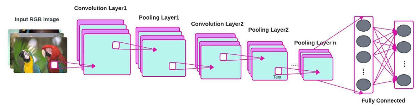
2.4. Background on convolution neural network in image
Architecture of convolution neural network, consist of input color image (RGB) then convolution this image with filter, then exchange all pixel less than zero to zero using ReLu layer, after that reduce the size of image to half by using pooling (max pooling or mean pooling), and the final layer (fully connected layer) applied (Zhao et al., 2024), as displayed in Figure 1.
2.4.1 Types of layers in CNN
1.Input layer
-
An image input layer is responsible for inputting two-dimensional images into an association while also implementing data normalization. Create an input layer labeled 'input' for 28-by-28 concealing images. Data normalization is executed by the layer through the elimination of the mean image of the structure set from each information image.
Picture input layer = picture input layer (input size, name, value)
A feature input layer: A part input layer inputs feature data to an association and applies data normalization. Use this layer when you have an educational assortment of numeric scalars tending to feature (data without spatial or time perspectives).
A feature input layer = feature input layer (numFeatures, ‘name,’ ‘value’)
2. Convolutional layer
In a CNN, the data is a tensor with a shape: (Number of data sources * input height * input width * input channels). Straightforwardly following going through a convolution layer, the picture becomes isolated to a part map, moreover, called an incitation map, with shape (number of data sources * feature map height * feature map width * consolidate guide channels). convolution channels to three layered data. The layer convolves the commitment by moving g the diverts along the data in a vertical heading, equally, and along the significance, managing the touch aftereffect of the heaps and the data, and a brief time later adding a tendency term.
Convolutional layer = convolution 3d layer (filter size, num filters, ‘name’, ‘value’).
3. Activation layers (Rectified Linear Unit (ReLU) layer)
In this layer we make a mask with the main image and its value is zero so that if the number in the main image is less than zero, the result will be zero, but if it is greater, it takes the value of the main image. A ReLU layer plays out an edge action to each part of the data, where any value under zero is set to nothing.
ReLU layer = ReLu layer ('name', ‘name’)
4. Pooling layer (max pooling, mean pooling)
This layer reduces the size of the main image in half by making a mean pooling mask that calculates for all the main image without adding new columns or rows so that it reduces its size in half.
There are two normal kinds of pooling in well-known use, max and mean. Max pooling utilizes the most extreme worth of every neighborhood bunch of neurons in the component map, while mean pooling takes the normal worth.
A three-layered max pooling layer performs down analysis by isolating three-layered commitment to cuboidal pooling areas, then, overseeing the constraint of each region.
Max pooling layer = max pooling 3d layer (pool size, ‘name’, ‘value’).
5.Mean pooling layer
A three-dimensional normal pooling layer performs down examination by partitioning three-layered contribution to cuboidal pooling locales, then, at that point, registering the normal upsides of every area.
Mean pooling layer = average pooling 3d layer (pool size, ‘name’, ‘value’).
6.Fully connected layer
Neurons in a completely associated layer have full connection with all beginnings in the past layer, as found in standard neural associations. It portrays them as only one segment for every one of the upsides of the framework or the principal picture with the goal that it is viewed as an entry to the neural organization.
A fully connected layer multiplies the input by a weight matrix and then adds a bias vector.
Fully connected layer = fully connected layer (output size, ‘name,’ ‘value’).
7. Output layers
Softmax layer: A softmax layer applies a softmax ability to the commitment, for request issues, a softmax layer and thereafter a gathering layer ordinarily follow the last related layer.
Softmax layer = softmax layer ('name','softmax1')
Classification output layer: A gathering layer calculates the cross-entropy adversity for request and weighted plan tasks with inconsequential classes.
Classification layer = classification layer ('name', 'output')
2.4.2. Types of padding:
Two types of padding are:
1. Valid padding
This type is harmful to the network and means that there is no padding in the network, i.e., keeping the image as it is incorrect and unmodified.
2. Same padding
It means adding padding to the grid with the same dimensions as the original image.
Algorithm of convolution neural network
3. Proposed methodology
In the methodology segment of this study, optimization, and DL techniques for adaptive image denoising are combined in a multifaceted fashion. The procedure begins by employing a CNN that has been pre-trained and is specifically customized for image-processing tasks. Denoise removal is executed independently on every color channel of the RGB images by CNN, which leverages its capability to identify intricate patterns and attributes in the data. The BOA is implemented as a method of optimization to accomplish adaptive denoising. By using this methodology, the adaptive weighted filter, which is vital to the denoising process, is enhanced.
Through the denoising process, for each color channel, the filter is optimized through the meticulous fine-tuning of PSNR-based goal functions. Speckled noise, a persistent issue in the field of image processing, is specifically targeted for resolution. The BOA, inspired by echolocation, uses a special behavior to help the AEWF better tell apart the important parts of an image from the background noise. The AEWF can effectively reduce noise caused by speckles by changing its settings based on the specific features of the image.
By combining Deep learning and optimization methods, this innovative approach creates a more powerful system than usual techniques for removing noise. The following sections will explain each step of this method in detail, and Figure 2 shows a graphical representation of the process. The proposed method for reducing noise works better and can be used in a wider range of situations because it can adjust to distinct levels of speckle noise. Indeed, let us proceed with an analysis of the procedural phases and furnish a written depiction of the methodology, accompanied by an elucidation of the proposed flowchart.
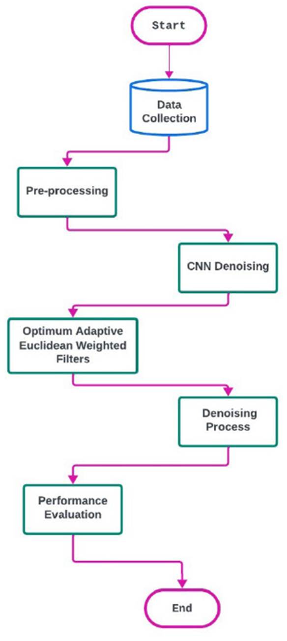
3.1.
Data acquisition: Please gather RGB images from the Kodak dataset that contain a variety of noise types
3.2.
Grayscale conversion of RGB images is required prior to processing. Speckle noise ought to subsequently be incorporated to replicate real-world conditions
3.3.
CNN-Denoising: Execute a CNN that has been modified for image processing-related tasks and has been previously trained. Proceed with the implementation of the CNN to remove noise from the RGB images on a per-channel basis
3.4.
AEWF One way to enhance the performance of an adaptive Euclidean weighted filter is through the implementation of the BOA algorithm. Following that, employ objective functions based on PSNR to adjust the filter parameters, thereby guaranteeing flexibility in handling different magnitudes of speckle noise and image attributes
3.5.
Denoising methodology: Composite the denoised color channels utilizing the adaptive weighted function (AWF). Following this, adaptive denoising can be achieved by modifying filter parameters flexibly in accordance with the image's characteristics. The BOA optimizes the parameters of the adaptive weighted filter in this section of the method to achieve the highest possible denoising performance for every color channel. The principal objective is to diminish speckle disturbance present in the image. Listed below is an explanation consisting of several distinct stages
3.5.6. Iteration optimization
Execute the solution update and bat moving steps frequently for a specified number of cycles, or until convergence is reached. The effective elimination of speckle noise in RGB images is made possible through the adaptive optimization procedure's utilization of the BOA and the Euclidean-weighted filter in the same direction.
The iterative process of the algorithm ensures continuous refinement of the filter parameters, thereby bolstering its ability to accommodate diverse noise conditions and augmenting the denoising efficacy.
4. Experimental results
Image quality is determined by the visual attributes of images and is dependent on the perceptual assessments of viewers. Typically, picture quality assessment strategies encompass subjective approaches that pertain to human perception, as well as realistic computational tools. The former approaches are better suited to our needs but often involve more time and money, whereas the latter methods are gaining recognition as the norm. Regrettably, these approaches often lack consistency due to the inherent limitations of objective methods in fully capturing the nuances of human visual perception. Consequently, significant disparities in outcomes might arise. Various performance evaluation criteria are employed in the process of denoising pictures. To conduct a thorough evaluation of image quality, the PSNR and SSIM are used based on the following formulas (Saleh et al., 2021).
Where
Case study 1
Case 1: In this case was used data input matrix X (4*4), matrix weight W (3*3) and filter (2*2).
By using applied algorithm CNN:
1. Convolution layer= X * Filter
2. ReLu layer: Max(0, X)
3. Pooling (2*2):
a)Max pooling (2*2)
b)Normal pooling (2*2)
4. Fully connected layer
5. V= W*X+B (A completely associated layer duplicates the contribution by a weight network and afterward adds a predisposition vector).
Case 2: For real-world evaluation, we utilized the KODAK dataset (Kodak dataset, n.d.), consisting of 24 images in PNG format, with sample images shown in Figure 3. The dataset is also an immensely popular validation dataset in the field of data compression. All images have dimensions of either 768x512 pixels or 512x768 pixels, depending on the orientation. Various levels of scatter noise were introduced, with variances of 0.01 in Figure 4, 0.05 in Figure 5, 0.1 in Figure 6, and 0.2 in Figure 7. These noises were subsequently removed using both conventional and proposed denoising techniques. PSNR and SSIM were computed for each method across different noise variances to assess their efficacy. Additionally, visual samples of the results were presented for comparative analysis. MATLAB 2022a software was employed for result acquisition, utilizing a computer system equipped with an Intel Xeon Silver 2.6 GHz processor, 16 GB RAM, and an NVIDIA GTX960M Quadro CPU.
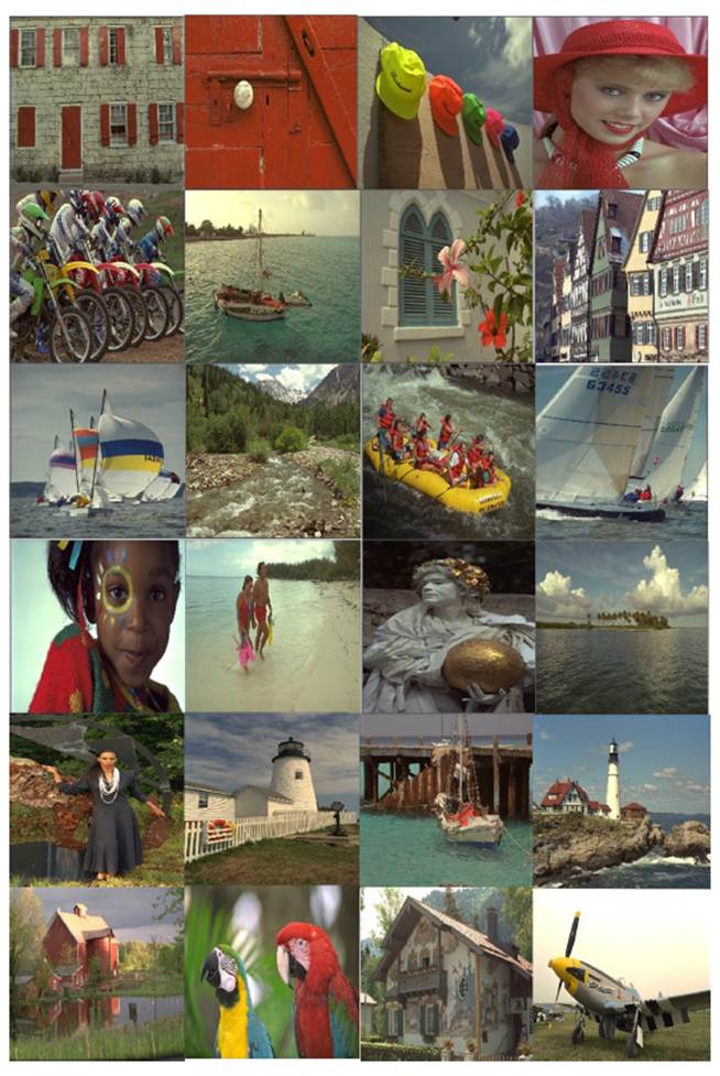
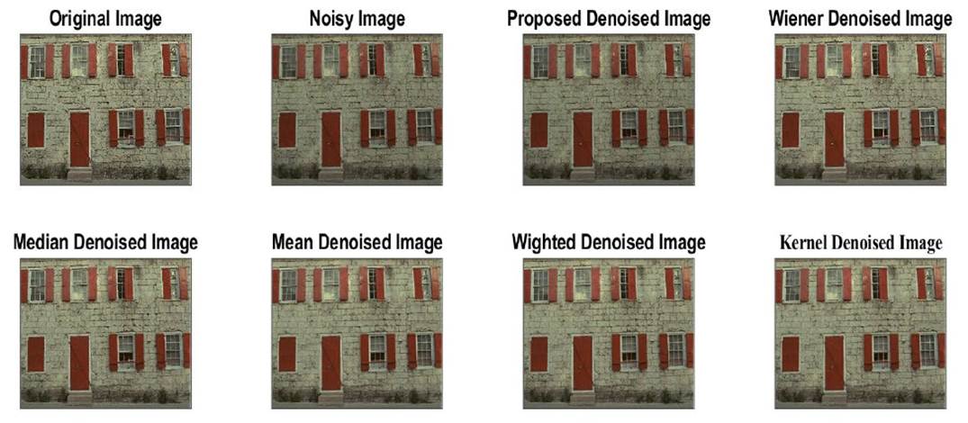
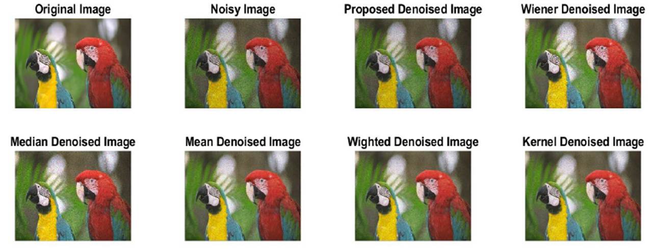
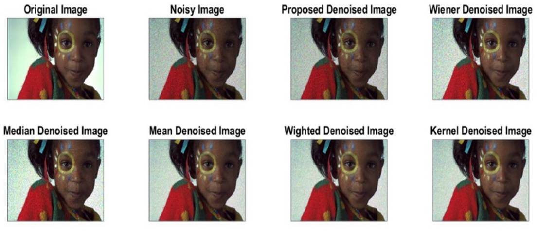
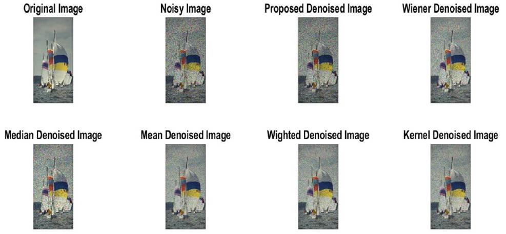
Table 1 shows the results of a study that compared various noise-reducing filters on images with varied levels of noise. With several metrics used to measure the filters' efficacy delineated in the columns, every row indicates a separate test instance. In particular, the metrics include the PSNR (peak signal-to-noise ratio) of the restored and source images. Notable findings include the suggested filter's persistently higher PSNR values compared to conventional filters such as Wiener, median, mean, weighted, and Kernel filters, which hold true across a wide range of noise intensities. The suggested filter shows remarkable resilience and the ability to effectively reduce noise without sacrificing image quality, as it continues to function exceptionally well even when faced with extremely high noise density. In contrast, the comparable filters' results vary depending on the level of noise, some of them showing reduced efficacy at greater densities. These results show that the suggested filter mechanism works, especially in difficult noise reduction situations, therefore it could be an effective way to tackle image denoising problems.
Table 1 PSNR values for speckle noise removal with a variance of 0.01: 0.2.
| No. | Noise density | Original PSNR | Wiener filter | Median filter | Mean filter | Weighted filter | Kernel filter | Proposed filter |
|---|---|---|---|---|---|---|---|---|
| 1 | 0.01% | 6.8537 | 25.8639 | 23.7811 | 23.3112 | 22.5576 | 23.3112 | 32.6834 |
| 2 | 0.01% | 9.9531 | 31.2783 | 28.4739 | 28.0307 | 27.5144 | 28.0307 | 32.6642 |
| 3 | 0.01% | 7.4344 | 29.5224 | 27.0414 | 26.8484 | 26.1570 | 26.8484 | 32.6617 |
| 4 | 0.01% | 7.7946 | 28.8295 | 26.8486 | 26.6536 | 25.9577 | 26.6536 | 32.8254 |
| 5 | 0.01% | 8.5821 | 27.7817 | 25.1449 | 24.1691 | 23.5525 | 24.1691 | 32.6053 |
| 6 | 0.05% | 4.8448 | 21.4418 | 18.6656 | 18.9848 | 18.1938 | 18.9848 | 32.5029 |
| 7 | 0.05% | 6.9155 | 22.5002 | 20.2212 | 20.4526 | 19.6209 | 20.4526 | 32.6204 |
| 8 | 0.05% | 5.3919 | 20.8404 | 18.3474 | 18.4139 | 17.7474 | 18.4139 | 32.4717 |
| 9 | 0.05% | 5.4389 | 20.6322 | 18.5943 | 18.8738 | 18.0495 | 18.8738 | 32.6609 |
| 10 | 0.05% | 6.0808 | 21.5016 | 19.2596 | 19.5484 | 18.7205 | 19.5484 | 32.6542 |
| 11 | 0.1% | 8.0400 | 20.8511 | 18.0400 | 18.3370 | 17.5799 | 18.3370 | 32.4539 |
| 12 | 0.1% | 3.6499 | 16.8498 | 14.6887 | 15.1213 | 14.4612 | 15.1213 | 31.9724 |
| 13 | 0.1% | 6.6040 | 20.0158 | 16.9607 | 17.2560 | 16.6153 | 17.2560 | 32.3727 |
| 14 | 0.1% | 7.6790 | 21.5644 | 18.1210 | 18.4216 | 17.7102 | 18.4216 | 32.4887 |
| 15 | 0.1% | 5.4914 | 22.4742 | 17.4554 | 18.0527 | 17.3864 | 18.0527 | 32.3282 |
| 16 | 0.2% | 7.1447 | 17.5360 | 14.6867 | 15.0912 | 14.5333 | 15.0912 | 31.5876 |
| 17 | 0.2% | 8.9406 | 20.3888 | 16.2306 | 16.6051 | 16.0826 | 16.6051 | 30.7463 |
| 18 | 0.2% | 9.9710 | 21.0264 | 17.6200 | 17.9714 | 17.3575 | 17.9714 | 32.9118 |
| 19 | 0.2% | 6.2633 | 16.8346 | 14.0513 | 14.4600 | 13.9943 | 14.4600 | 29.6158 |
| 20 | 0.2% | 2.3361 | 16.4520 | 12.8719 | 13.7746 | 13.3868 | 13.7746 | 28.3319 |
An experiment was conducted to compare several noise reduction filters applied to images with varying levels of noise density. The results are presented in Table 2. The columns show several metrics that evaluate the filters' performance, and each row represents a separate test instance. The suggested filtered consistently outperforms other methods in preserving structural similarity between restored and source images, as shown by its consistently high Structural Similarity Index (SSIM) values across different noise intensities. That the suggested filter technique successfully lowers noise levels without degrading the image's quality
Table 2 SSIM values for speckle noise removal with a variance of 0.01: 0.2.
| No. | Noise density | Original SSIM | Wiener filter | Median filter | Mean filter | Weighted filter | Kernel filter | Proposed filter |
|---|---|---|---|---|---|---|---|---|
| 1 | 0.01% | 0.0073 | 0.6904 | 0.6153 | 0.5882 | 0.4965 | 0.5882 | 0.9836 |
| 2 | 0.01% | 0.0182 | 0.7185 | 0.6481 | 0.6377 | 0.5588 | 0.6377 | 0.9825 |
| 3 | 0.01% | 0.0178 | 0.6723 | 0.5774 | 0.5659 | 0.4708 | 0.5659 | 0.9815 |
| 4 | 0.01% | 0.0146 | 0.6637 | 0.5898 | 0.5798 | 0.4849 | 0.5798 | 0.9830 |
| 5 | 0.01% | 0.0111 | 0.7909 | 0.7506 | 0.7121 | 0.6528 | 0.7121 | 0.9826 |
| 6 | 0.05% | 0.0076 | 0.5463 | 0.3628 | 0.3456 | 0.2094 | 0.3456 | 0.9858 |
| 7 | 0.05% | 0.0112 | 0.5804 | 0.4235 | 0.4062 | 0.2801 | 0.4062 | 0.9852 |
| 8 | 0.05% | 0.0061 | 0.5955 | 0.4777 | 0.4532 | 0.3469 | 0.4532 | 0.9859 |
| 9 | 0.05% | 0.0111 | 0.4786 | 0.3191 | 0.2984 | 0.1529 | 0.2984 | 0.9847 |
| 10 | 0.05% | 0.0119 | 0.4848 | 0.3279 | 0.3095 | 0.1632 | 0.3095 | 0.9842 |
| 11 | 0.1% | 0.0191 | 0.5698 | 0.3674 | 0.3530 | 0.2255 | 0.3530 | 0.9856 |
| 12 | 0.1% | 0.0088 | 0.4524 | 0.2513 | 0.2243 | 0.0987 | 0.2243 | 0.9852 |
| 13 | 0.1% | 0.0051 | 0.5467 | 0.3679 | 0.3568 | 0.2374 | 0.3568 | 0.9862 |
| 14 | 0.1% | 0.0133 | 0.5886 | 0.3946 | 0.3825 | 0.2631 | 0.3825 | 0.9851 |
| 15 | 0.1% | 0.0278 | 0.6033 | 0.3819 | 0.3657 | 0.2446 | 0.3657 | 0.9861 |
| 16 | 0.2% | 0.0105 | 0.4640 | 0.2452 | 0.2253 | 0.1064 | 0.2253 | 0.9832 |
| 17 | 0.2% | 0.0341 | 0.5721 | 0.3554 | 0.3426 | 0.2343 | 0.3426 | 0.9819 |
| 18 | 0.2% | 0.0149 | 0.5291 | 0.3555 | 0.3453 | 0.2210 | 0.3453 | 0.9859 |
| 19 | 0.2% | 0.0089 | 0.4715 | 0.2643 | 0.2413 | 0.1387 | 0.2413 | 0.9829 |
| 20 | 0.2% | 0.0099 | 0.5189 | 0.2558 | 0.2391 | 0.1493 | 0.2391 | 0.9868 |
is supported by the results. In contrast, the efficiency of other filters-including the Kernel, median, mean, weighted, and Wiener filters-varies with the quantity of noise. The suggested filter maintains reliable results even at larger noise density levels, in contrast to other filters that have trouble maintaining the image's quality as the level of noise increases from 0.01% to 0.20%. All filters work well at a lower level of noise (0.01% and 0.05%). These findings indicate that the suggested filter technique can be successful, especially in difficult reduction of noise situations, and that it could be a good strategy for image noise reduction.
The SSIM and PSNR metrics are essential in assessing the effectiveness of denoising methods, providing unique viewpoints on the evaluation of image quality. Quantifying reconstruction accuracy, PSNR evaluates the fidelity of the reconstructed image in comparison to the original through the calculation of the peak signal-to-noise ratio. On the other hand, SSIM assesses the degree of structural similarity between the original and denoised images by taking perceptual factors including contrast, luminance, and structure into account. In contrast to PSNR, which is sensitive to changes in pixel values and provides a quantitative measure of the effectiveness of noise reduction, SSIM provides a more comprehensive evaluation by integrating human visual perception.
It is essential to recognize the interaction between several evaluation metrics, such PSNR and SSIM, while assessing denoising approaches. Consider the possibility that artifacts may be introduced that have a detrimental effect on SSIM scores if PSNR augmentation is prioritized, and vice versa. To get the desired noise reduction outcomes, it is crucial to achieve a suitable equilibrium among these measures. Our work involved numerical analyses that utilized our framework to measure the effect of various denoising techniques on PSNR and SSIM values. Based on the tables that were provided, our results show some interesting insights. To illustrate its effectiveness in maintaining structural similarity between restoration and source images, the suggested filter routinely beats various others based on SSIM across different noise levels, as shown in Table 1. On the other hand, our suggested technique outperforms the current filters by 0.1 SSIM and 5 dB in overall PSNR, as shown in Table 2 of the numerical research. The results show that our strategy achieves a good compromise between visual quality and subjective performance, as seen by the PSNR and SSIM metrics that increase. Incorporating imagine identification tasks into our research further supports the relevance of denoising approaches combining perception efficiency with restoration accuracy, as seen in the tables presented. The enhanced accuracy in image identification tasks that may be achieved by denoising algorithms that optimize both PSNR and SSIM values highlights the practicality of this method. This subsection delves further into these trade-offs, illuminating the complex interplay between signal-to-noise ratio (SNR), signal-to-noise ratio (SSIM), and image identification accuracy. Our goal is to help researchers and professionals improve the functionality of image processing applications by demystifying these complexities and basing their conversation on numerical calculations to our framework. This will allow them to create denoising techniques that successfully balance perception characteristics with restoration precision.
5. Conclusion
This research study presents a novel approach to image restoration that combines DL with the bat optimization algorithm (BOA) to enhance the performance of a weighted adaptive filter. Our technique, known for its versatility in handling different speckle noise circumstances, outperforms traditional denoising filters. By integrating a pre-trained convolutional neural network (CNN) specifically designed for removing noise from color channels, we guarantee reliable and accurate pattern identification. Additionally, the BOA algorithm constantly adapts the settings of the AEWF method to efficiently minimize speckle noise. Our results show that noise reduction efficiency has been significantly improved through extensive computation and experimental testing. Our technique outperforms traditional filters in noise reduction, as it regularly produces superior PSNR and SSIM ratios. Our method outperformed state-of-the-art filters in terms of overall PSNR enhancement (5 dB) and SSIM enhancement (0.1), according to the results of our studies. A flowchart graphically depicts the intricate interaction of CNNs, BOA, and AEWF, and the organized parts of the paper provide an exhaustive description of each process step. This approach has enormous promise for enhancing picture quality and decreasing speckle noise issues in a wide range of applications, thanks to the continuous development in image processing techniques.

