


 nueva página del texto (beta)
 Inglés (pdf)
 Artículo en XML
 Referencias del artículo
 Enviar artículo por email
 Citado por SciELO
  Similares en
SciELO
Similares en
SciELO 
 Permalink
1 Introduction
Breast cancer is one of the most dangerous types of cancer among women around the world. It is also one of the leading causes of mortality in middle and old aged women. The World Health Organization’s International Agency for Research on Cancer estimates that more than 1 million cases of breast cancer will occur worldwide annually, with 580,000 cases occurring in developed countries and the remainder in developing countries. The risk of a woman developing breast cancer during her life time is approximately 11% [1]. The early detection of breast cancer is of vital importance for the success of treatment, with the main goal to increase the probability of survival for patients. Currently the most reliable and practical method for early detection and screening of breast cancer is mammography. Microcalcifications can be an important early sign of breast cancer, these appear as bright spots of calcium deposits. Individual microcalcifications are sometimes difficult to detect because of the surrounding breast tissue, their variation in shape, orientation, brightness and diameter size [2]. Microcalcifications are potential primary indicators of malignant types of breast cancer, therefore their detection can be important to prevent and treat the disease. In this paper, an effective methodology in order to detect Microcalcifications in digitized mammograms is presented. This approach is based on the synergy of Image Processing, Pattern Recognition and Artificial Intelligence. But it is still a hard task to detect all the Microcalcifications in mammograms, because of the poor contrast with the tissue that surrounds them.
However, many techniques have been proposed to detect the presence of microcalcifications in mammograms: image enhancement techniques, Artificial Neural Networks, wavelet analysis, Support Vector Machines, mathematical morphology, image analysis models, fuzzy logic techniques, etc. Image enhancement algorithms have been utilized for the improvement of contrast features and the suppression of noise. In [3] proposed five image enhancement algorithms for the detection of microcalcifications in mammograms.
Bhattacharya and Das [4], proposed a method based on discrete wavelet transform due to its multiresolution properties with the goal to segment microcalcifications in digital mammograms. Morphological Top-Hat algorithm was applied for contrast enhancement of the microcalcifications. Fuzzy C-Means clustering algorithm was implemented for intensity-based segmentation. Sung et al. [5], proposed an approach by means of mathematical morphology operations and wavelet transform to locate the microcalcifications in digital mammogram.
In [6] proposed an algorithm that was tested over several images taken from the digital database for screening mammography for cancer research and diagnosis, and it was found to be absolutely suitable to distinguish masses and microcalcifications from the background tissue using morphological operators and then extract them through machine learning techniques and a clustering algorithm for intensity-based segmentation. Segmentation processes for the detection of textures, ROIs, lesions, tumors have also been used on photo-acoustic images [7] and thermographic images [8].
The remaining sections of this work are organized as follows: Section 2, presents the details of the proposed method. Section 3, presents the details of the proposed method and experimental results while the conclusions are presented in sections 4, respectively.
2 Methodology
2.1 Image Selection
The images used to train and test this methodology were extracted from the mini-mammographic database provided by the Mammographic Image Analysis Society, MIAS [17]. Each mammogram from the database is 1024×1024 pixels and with a spatial resolution of 200 micron pixel edge. These mammograms have been reviewed by an expert radiologist and all the abnormalities have been identified and classified. The place where these abnormalities such as Microcalcifications, have been located is known as, Region of Interest (ROI). The ROI size in this work is 256×256 pixels.
2.2 ROI Enhancemen
The difficulty for the detection of Microcalcifications depends on some factors, such as, size, shape and distribution with respect to their morphology. On the other hand the Microcalcifications are often located in a non-homogeneous background and due to their low contrast with the background, its intensity may be similar to noise or other structures [9-10]. In this paper, the goal of image enhancement is to improve the contrast between the Microcalcifications clusters and background, for achieving this task morphological operations based on Coordinate Logic Filters (CLF) are implemented.
Mathematical Morphology is a discipline in the field of image processing which involves an analysis of the structure of images. The geometrical structure of image is determined by locally comparing it with a predefined elementary set called structuring element. Image processing using morphological transformations is a process of information removal based on size and shape, in this process irrelevant image content is eliminated selectively, thus the essential image features can be enhanced. Morphological operations are based on the relationships between the two sets: an input image, G, and a processing operator, the structuring element, SE, which is usually much smaller than the input image. By selecting the shape and size of structuring element, different results may be obtained in the output image. The fundamental morphological operations are: erosion and dilation.
CLF were proposed in [11], and constitute a class of non-linear digital filters that are based on the application of Coordinate Logic Operations (CLO) to a single image as dictated by a SE, where CLO are the basic logic operations (NOT, AND, OR, and XOR, and their combinations). CLF are very efficient in digital signal processing applications, such as noise removal, magnification, skeletonization, coding, edge detection, feature extraction, fractal modelling and can execute the morphological operations (erosion, dilation, opening and closing) and the successive filtering and managing of the residues. The execution of CLO (AND, OR) in CLF is performed on the binary values of the image pixels and are analogous to the execution of (MIN, MAX) in the morphological filters. That makes the CLF have analogous operability with the corresponding morphological ones. Moreover, CLF satisfy all the corresponding morphological properties except the increasing property. The CLF coincide with morphological filters in the case of binary images. They could also coincide with gray-scale morphological filters provided that images are quantized and mapped on a specific set of decimal values [5]. Given a gray level image G, the decomposition in a set of binary images S_k,k=0,1,…,n-1, according to the decomposition of the (i,j) pixel, is denoted by:
where
The contrast can be defined as the difference in intensity between an image structure and its background. By combining morphological operations, several image processing tasks can be performed, but in this work morphological operations are used to achieve contrast enhancement. In [12], the contrast enhancement technique using mathematical morphology is called morphological contrast enhancement. Morphological contrast enhancement is based on morphological operations known as top-hat and bottom-hat transforms. A Top-Hat is a residual filter which preserves those features in an image that can fit inside the structuring element and removes those that cannot in other words the Top-Hat transform is used to segment objects that differ in brightness from the surrounding background in images with uneven background intensity. The Top-Hat transform is defined by the following equation:
where G is the input image, G_T is the transformed image, SE is the structuring element, ⊖ represents morphological erosion operation, ⊕ represents morphological dilation operation and - image subtraction operation. [(G⊖SE)⊕SE] is also known as the morphological opening operation.
2.3 Image Segmentation by Clustering Algorithms
Image segmentation is an important task in the field of image processing and computer vision and involves identifying objects or regions with the same features in an image. The purpose of image segmentation is to subdivide an image into non-overlapping, constituent regions which are homogeneous with respect to some features such as gray level intensity or texture. The level to which the subdivision is carried out depends on the problem being solved [13]. In the field of medical imaging, segmentation plays an important role because it facilitates the delineation of anatomical structures and other regions of interest. For the specific case as Microcalcifications detection, several works based on image segmentation by means of clustering algorithms have been proposed [14-16]. In this work, for the image segmentation stage, two techniques based on partitional clustering algorithms are used. The aim of this stage is to segment the ROI images to make easier the Microcalcifications detection. The algorithms used in this stage are k-means and SOM.
k-means is one of the simplest unsupervised learning algorithms that solve the well known clustering problem. The procedure follows a simple and easy way to classify a given data set
where
where
The neurons of the Kohonen layer compete to see which neuron will be stimulated by the feature vector
The neighbourhood function or Gaussian function determines how much the neighbouring neurons become modified. Neurons within the winners neighbourhood participate in the learning process. During the self-organizing process, the neighbourhood size decreases until its size
2.4 Classification of Microcalcifications by AMMLPs
Artificial Neural Networks (ANNs) are used in a wide variety of data processing applications where real-time data analysis and information extraction are required. One advantage of the ARTIFICIAL NEURAL NETWORKS approach is that most of the intense computation takes place during the training process. Once ANNs are trained for a particular task, their operation is relatively fast and unknown samples can be rapidly identified in the field.
In this work, Artificial Metaplasticity (AMP) is applied to the learning algorithm of a Multi-Layer Perceptron. Metaplasticity is a biological concept related to the way information is stored by synapses in the brain. Artificial metaplasticity was recently proposed in [17], where it is modelled by giving more importance to less frequent patterns in the training process. One advantage of the use of AMP is that it usually results in a more efficient training because a small set of training patterns is usually required. This approach is in fact equivalent to the application of importance sampling to artificial neural networks training [18].
In the classic backpropagation algorithm the learning rate is usually fixed for all input patterns meaning that it gives the same importance to all patterns. AMP can be included in the training process by simply introducing a weighting function
Ideally, the function
where N is the dimension of the input vector X (for the second hidden layer, X is substituted by the output vector of the first hidden layer, and so on) and
3 Results
The proposed methodology is applied to each of the ROI images individually in order to show the obtained results by means of a segmented image. Several ROI images with dense tissue and the presence of Microcalcifications were selected to train and test the proposed methodology. The morphological Top-Hat transform is used in order to enhance the ROI image, with the goal of detecting objects that differ in brightness from the surrounding background, in this case the goal is to increase the contrast between the Microcalcifications and the background. The size of each SE used is
In the next stage two window-based features such as, mean and standard deviation are extracted from enhanced images within a rectangular pixel window of size
Next, a Feature Vector (FV) for each ROI image is built, a set of FVs is formed for each obtained image from the previous process. First, a mapping is performed from the gray level intensity to a vector as follows:
In this work, criterions were used to determine which cluster represents an MC group: minimum number of data clustered into class with maximum gray level value as well as the clusters separability approach. A between-class dispersion matrix
The initial conditions for the segmentation and results for each clustering method are presented next. For k-means: the number of clusters takes values from 2 to 6, cluster centers are initialized randomly, Euclidean distance is used and the maximum number of iterations is 100.
The initial conditions for the SOM are: the network structure is
Table 1 shows the number of patterns assigned to classes
Table 1 Number of patterns assigned to Q1 an Q0
| Label | Number of patterns by k-means |
Number of patterns by SOM |
|---|---|---|
| Q0 | 588181 | 583081 |
| Q1 | 1643 | 6743 |
Due to the large amount of patterns that do not belong to Microcalcifications with respect to the number of patterns that belong to Microcalcifications a balancing was performed, see Table 2.
Table 2 Results of balancing
| Label | Number of patterns by k-means | Number of patterns by SOM |
|---|---|---|
| Q0 | 8215 | 33715 |
| Q1 | 1643 | 6743 |
To comparatively evaluate the performance of the classifiers, all the classifiers presented in this particular case were trained with the same training dataset and tested on the same testing dataset. In order to determine the neural network structure and metaplasticity parameters, the same network parameters as applied in [23] and [17], were used. Table 4 shows the metaplasticity parameters
Table 3 Number of patterns used for training and testing
|
|
Number of Samples | Total | ||
|---|---|---|---|---|
| Training | Testing | |||
| k-means |
|
1160 | 483 | 1643 |
|
|
5741 | 2474 | 8215 | |
| SOM |
|
5413 | 1330 | 6743 |
|
|
26954 | 6761 | 33715 | |
Table 4 The best neural network structures and metaplasticity parameters
| Data Set |
Neural Network Structure |
Metaplasticity Parameters |
Mean Squared |
|||
|---|---|---|---|---|---|---|
| I | HL | O | A | B | Error | |
| k-means | 4 | 15 | 1 | 39 | 0.5 | 0.01 |
| 4 | 12 | 1 | 39 | 0.5 | 0.01 | |
| SOM | 4 | 15 | 1 | 39 | 0.25 | 0.01 |
| 4 | 10 | 1 | 39 | 0.5 | 0.01 | |
In our work different network structures were used; the activation function is a sigmoid; and with the same metaplasticity parameters. Table 4 shows the best network structure and metaplasticity parameters for each FV.
A confusion matrix is built to determine the probability of false detection. Table 5 shows the performance of the classifiers presented in this work as well as the corresponding confusion matrices. As it can shown, the best accuracy (99.93%) and specificity (99.95%) are obtained for a SOM and an AMMLP with a [4:15:1] structure. The second best accuracy (99.78%) and specificity (99.94%) are also obtained for a SOM and an AMMLP. However, the best sensitivity (100%) is obtained for k-means and an AMMLP with a [1:15:1] structure.
Table 5 Confusion matrices and performance of the classifiers
| AMMLP Structure |
Desired Results |
MC | Output Results Normal Tissue |
Sensitivity (%) |
Specificity (%) |
Accuracy (%) |
|---|---|---|---|---|---|---|
| k-means | ||||||
| 4:15:1 | MC | 483 | 0 | 100 | 99.67 | 99.72 |
| Normal Tissue |
8 | 2466 | ||||
| 4:12:1 | MC | 476 | 7 | 98.55 | 99.63 | 99.45 |
| Normal Tissue |
9 | 2465 | ||||
| SOM | ||||||
| 4:15:1 | MC | 1328 | 2 | 99.84 | 99.95 | 99.93 |
| Normal Tissue |
3 | 6758 | ||||
| 4:10:1 | MC | 1317 | 13 | 99.02 | 99.94 | 99.78 |
| Normal Tissue |
4 | 6757 | ||||
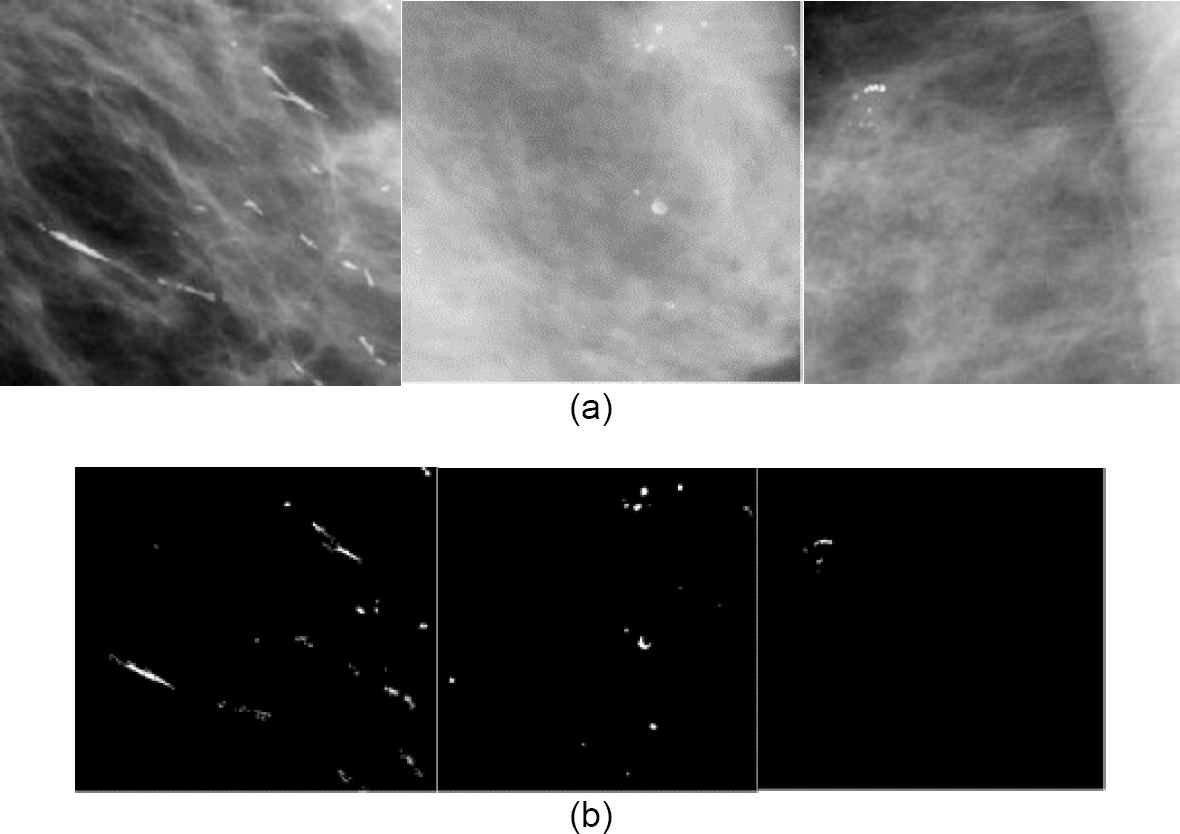
Finally, Figure 1 shows examples of the obtained results of the detection of Microcalcifications using the methodology proposed in this paper.
4 Conclusion
In this work a system for microcalcification detection was proposed based on two clustering algorithms, k-means and Self Organizing Maps, Coordinate Logic Filters and a neural network based on Artificial Metaplasticity. Clustering algorithms help us get a better comprehension and knowledge of the data with the objective of segmenting the image into different areas (background and MC). Before applying the clustering algorithms, we applied a digital image processing technique for image enhancement using mathematical morphology operations in order to improve the contrast between Microcalcifications and the background in the ROIs. One advantage of mathematical morphology operations based on Coordinate Logic Filters is due to their easy hardware implementation, although in this work only simulation was carried out. The AMMLP classifier plays an important role in our methodology because ARTIFICIAL NEURAL NETWORKS can learn structure in data through examples contained in a training set and then can conduct complex decision making. From the obtained results, we conclude that the proposed system constitutes a promising approach for the detection of Microcalcifications. The experimental results show that the proposed methodology can locate Microcalcifications in an efficient way.

