


 nueva página del texto (beta)
 Inglés (pdf)
 Artículo en XML
 Referencias del artículo
 Enviar artículo por email
 Citado por SciELO
  Similares en
SciELO
Similares en
SciELO 
 Permalink
1. Introduction
1.1 General climatological background
The negative impacts of climate change are increasingly noticeable and accentuated in all regions of the planet. The global increase in temperature has intensified the hydrological cycle, increasing the number of extreme weather phenomena (IPCC, 2023). These hydro-meteorological processes are commonly related to a greater frequency and intensity of hurricanes, or to the increase of dry seasons and the delay of the rainy season, among other consequences. According to Quante et al. (2021), the increase in air temperature results in higher evaporation rates and, therefore, a greater potential for precipitable water; at the same time, a higher temperature causes a decrease in snowfall occurrence, increasing the volume of liquid precipitation. This relationship between the increase in air temperature and the decrease in snow precipitation has been analyzed in future scenario models (Pons et al., 2016). Notwithstanding the above, severe winter storms have occurred more frequently, mainly in mid-latitude countries of Europe and the United States, and like other extreme hydro-meteorological phenomena, they are capable of halting commercial, industrial, and social activities in the affected regions, causing severe damage to the economy and infrastructure, and causing fatalities in extreme cases (NOAA, 2017). This seems to align with Quante et al. (2021), who, using projection models, predicted that heavy snowfall occurrence will increase mainly in North America and Asia in the coming decades.
North American winter conditions are generally governed by the movement of polar air masses into regions outside their regular boundaries. Cyclical processes such as El Niño Southern Oscillation (ENSO), the Pacific Decadal Oscillation (PDO), the Madden Julian Oscillation (MJO), the Quasi Biennial Oscillation (QBO), the Artic Oscillation (AO), the North Atlantic Oscillation (NAO), and the Eastern Pacific Oscillation (EPO) appear to influence, both by their temperature and humidity characteristics, the magnitude of winter weather in the American boreal hemisphere (Frontier Weather, n.d.), as they combine with the displacement of Arctic polar air masses. As an example of the above, Woollings et al. (2010) mention that NAO is a component that, together with ENSO and the MJO (Cassou, 2008), largely determines the latitudinal displacement of the jet stream and, therefore, of the polar frontal system.
The polar boundary between Farrel and Polar cells gives rise to the jet stream at the limits of the tropopause, circling the planet with small undulations in a west-east trajectory and decreasing in latitude during the winter, while in the summer it is located closer to the poles (Shapiro and Keyser, 1990). This boundary controls the horizontal position of the polar front, separating the regions of warm subtropical and temperate air from the cold Arctic mass as it moves around the circumpolar regions of the planet.
The polar vortex is bounded by a higher velocity of the jet stream during the winter, while its velocity tends to decrease during summer. However, the increasing influence of warm air masses towards the polar regions, even during the winter, may cause a lower horizontal temperature gradient between the air masses on both sides of the jet (Woollings et al., 2023). At the same time, the convective ascent of energy to the stratosphere, above the cell boundary, causes the weakening and slowing of the jet stream, which gives rise to the formation of Rossby waves, causing the formation of meanders that can reach great amplitude, sometimes reaching latitudes as low as the southern United States. Rossby waves develop a cyclonic circulation inside the lower part of the wave, while inside the upper part they originate a high-pressure anticyclonic system. Sometimes, the weakening causes the jet circulation to remain almost stationary for several days in some places; then, the cyclonic system inside the wave (positive vorticity) will generate adverse winter weather conditions due to the stagnation of polar air (the polar vortex itself) causing the persistence of freezing temperatures and severe winter storms during its permanence (Stendel et al., 2021).
Future scenario models indicate a greater frequency of sudden stratospheric warmings (Wills et al., 2019), causing the slowing of the jet and consequently generating the elongation of the polar vortex towards mid-latitudes. Stendel et al. (2021) even mention a growth rate in the amplitude of the wave of up to 20 m yr-1, bringing with it increasingly severe winter episodes at lower latitudes (Mitchell et al., 2012). When polar air masses move from their source regions, they change weather conditions during their transfer and modify their own characteristics through the exchange of temperature and humidity (Spiridonov and Ćurić, 2021).
Commonly, the displacement of cold air masses begins across Canada and the United States, reaching northern and central Mexico (Lagerquist et al., 2020), with temperature conditions cold enough even to cause periods of thermal decline during its passage. If the temperature falls below the freezing point and the humidity conditions are favorable, snowfall will occur. These winter weather effects may be more severe, which will cause greater elongation and stagnation of the jet meanders.
Smith and Sheridan (2018) identified 49 periods of extreme cold in the east-central United States between 1948 and 2016, with an average duration of six days; however, they recorded episodes exceeding 20 days in duration and temperature values as low as -22 ºC, which have involved more than 20 major cities. A recent case occurred on February 10 and 18, 2021, when winter storm Uri impacted 25 US states. Texas, one of the southernmost states, was the region of greatest impact (Nejat et al., 2022), recording a temperature of -18 ºC (Veettil et al., 2022), when the average minimum values during winter are around 0 ºC. Uri left behind a snow accumulation of 16 cm (ATC, 2021). The repercussions of this storm reached Mexico between February 13 and 19, with the arrival of the cold front 36, which left severe snowfall in the states of Sonora, Chihuahua, Coahuila, Nuevo León, and Tamaulipas, where temperatures reached as low as -15.5 ºC, while in states of the central region such as Guanajuato, Jalisco, Michoacán, Morelos, Mexico, and Veracruz, values between -2.9 and -9 ºC were recorded, with snowfall and severe frosts in mountainous regions above 2500 masl (CONAGUA, 2021). Beyond service system failures and economic losses, the most serious consequence was the number of victims due to hypothermia, as well as carbon monoxide (CO) poisoning. In some places, these cases became fatal (El Mundo de Hoy, 2021; Le Duc and Villalpando, 2021).
The characteristics of the Mexican relief, from sea level up to 5610 masl, favor different climates, ranging from warm and humid to cold and dry, as well as a wide biodiversity. The most contrasting region, due to elevation and climate, is located at the eastern end of the Neovolcanic Axis in the center of the state of Veracruz. Here, starting from the coastline, the terrain’s altitude steadily increases until it reaches a natural barrier separating the windward slope from the Mexican Plateau (Soto and Cervantes, 2023). Three of the highest mountains in the country are located at the ends of this barrier. Because of its climatological, geomorphological, and edaphic conditions, this region has great agricultural and livestock potential, which determines, among other factors, the existence of many rural settlements. However, due to the freezing conditions to which inhabitants are exposed during winter, vast areas have been documented over several decades with crop loss, as well as numerous cases of deaths (Zermeño-Díaz et al., 2021), which, among other causes, are a consequence of the vulnerability of many of these populations (Jáuregui et al., 2020).
1.2 Health vulnerability to extreme cold
Vulnerability is the susceptibility or propensity of an affectable agent to suffer damage or loss in the presence of a disturbing process, determined by physical, social, economic, and environmental factors (SEMARNAT, 2023). It has been commonly associated with population characteristics such as gender, age, schooling, health, income, and housing type (Sosa-Capistrán and Vázquez-García, 2014; Travieso-Bello et al., 2018). In a population vulnerable to extreme cold, exposure to extremely low temperatures may cause hypothermia (when body heat is less than 35 ºC) since the body loses heat by physical principles; that is, by radiation, convection, conduction, and evaporation (which together form thermoregulation); therefore, prolonged contact with water or a cold atmosphere may represent an increased risk of hypothermia, which may range from mild (32-35 ºC) to severe (less than 28 ºC).
In inhabited regions with intense cold conditions, whether permanent or seasonal, the population suffers anatomical and metabolic changes because of exposure to low temperatures and little sun exposure (Ramón et al., 2023). Newborns, pregnant women, and older adults are the age groups with the greatest health vulnerability to severe winter conditions, which happens mainly due to natural immunosuppression derived from young age, pregnancy, and cellular senescence, respectively (Castelo-Branco y Soveral, 2014; Müller et al., 2019). This process causes the susceptibility of the mentioned age groups to the development of opportunistic microorganisms and the evolution of severe complications. Even in healthy adults, where low temperatures require shorter periods for vasoconstriction and vasodilatation to maintain vital temperature, it has repercussions on blood pressure changes and increases the risk of atheroembolism (Abrignani et al., 2022). Hypothermia is commonly associated with decreased blood flow to the brain and low oxygen consumption. Many deaths usually occur once a severe decrease in brain function occurs (Vargas-Téllez, 2009).
In severe cold conditions, the most marginalized populations commonly make use of wood fires for heating and cooking, whose combustion produces noxious gases that, when chronically inhaled, change the morphology of lung tissue, increasing the risk of chronic obstructive pulmonary disease (COPD), bronchial diseases, and lung cancer; they also trigger asthma attacks, which increase the morbidity and mortality rate (Zhang et al., 2021). The consequences, even fatal, become immediate when intoxication or asphyxiation by CO inhalation occurs indoors (Tortorella and Laborde, 2021). In summary, in the face of severe winter cold conditions, the most vulnerable populations (strongly related to their level of marginalization) are susceptible to numerous physiological alterations derived from climatological and social conditions (Hajat, 2017), where the combination of low temperatures and marginalized conditions are determinants for population health and limit the development of a healthy life.
Considering that in Mexico there are only a few weather stations in mountain environments (Soto and Delgado, 2020) and little is known about the distribution of frost and snowfall occurrence in high-mountain regions (Soto and Delgado-Granados, 2024), and also taking into account the strategic location of the Pico de Orizaba-Cofre de Perote mountain range, its elevation, fertility of soils, and the number of inhabitants surrounding the area, the main objective of this work is to determine the area of freezing, both due to frost and snowfall, that occurred during the winter of 2021-2022. The results suggest using a proposed methodology that partially compensates for the lack of weather stations in Mexican high mountains and, at the same time, allows modeling the freezing surfaces, which is somewhat common in the country’s high mountainous relief during most winters. Moreover, it allows us to analyze the number of populations and inhabitants exposed to severe freezing conditions, which can severely affect their health, directly or indirectly.
2. Methodology
2.1 Study area
The Neovolcanic Axis runs horizontally across the country’s central part and comprises numerous monogenetic and stratovolcanoes. At its eastern end lies the highest point in the country, the Citlaltépetl volcano, which reaches 5610 masl. The Sierra Negra volcano (4580 masl) and the Cofre de Perote (4200 masl), located approximately 100 km to the north, are also part of this axis. The small mountain range that connects these peaks exceeds 3000 masl. This orographic ridge represents the main watershed that divides the slope of the Gulf of Mexico and the Mexican Central Plateau, as well as the border between the states of Puebla and Veracruz. The areas on either side of the ridge have contrasting climates and different types of ecosystems. The soils of this mountainous strip, being of volcanic origin, are rich in minerals; at the same time, the continuous condensation of atmospheric humidity, in response to the upward forcing of the air along the windward slope, makes it an important rain and water catchment area; the combination of the above favors the agricultural and livestock activities of the place, which are a fundamental part of its economy.
According to Soto and Cervantes (2023), the Foehn effect determines that the eastern slope has a temperate and humid climate, with the highest concentration of precipitation located around 1500 masl, with an average accumulated value of 2000 mm, although there are sites that exceed 2500 mm per year. The average temperature ranges from 4.6 to 8.2 ºC during the month of January, while in July, it ranges from 5.7 to 11.5 ºC on average. In the peaks of Citlaltépetl and Cofre de Perote, temperatures during January are -2.9 and 3.8 ºC respectively, as well as -2.4 and 5.5 ºC during July (Fernández-Eguiarte et al., 2010). On the opposite slope, the drying ratio, together with the Foehn effect, determine a rainfall index lower than that of the windward slope, causing a large part of the Central Plateau, with an average altitude of 2200 masl, to register an accumulated precipitation regime of less than 1000 mm per year. During the winter season, the arrival of cold air masses is frequent in the area since, of the total number of frontal systems that enter the country each year (~50), more than half reach the central region and the study area, being more noticeable during January (CONAGUA, 2023). As they pass through, they cause mild to cold temperatures depending on the height of the relief, with precipitation mostly observed on the eastern slope of the orographic barrier, as well as north and northeast winds.
The vegetation on both slopes differs. The climate is temperate and humid on the windward side, which favors the existence of a mesophyll forest, which reaches its upper limit at approximately 2500 masl. The pine and conifer forest continues from this elevation until reaching 4060 masl (Soto and Welsh, 2023). At this point, the scrubland begins, interspersed with soil and bare rock in the highest parts of the main summits. The vegetation on the leeward slope transitions from pine and coniferous forest at higher elevations to mostly shrub and bush cover at lower elevations (Soto et al., 2021). Similarly, agricultural activities involve the use of land for grazing cattle and sheep, as well as for growing crops such as coffee, corn, and vegetables. The study region occupies a total area of 2949 km2 and is defined by the 2400 isohypse, which marks the lower limit and perimeter of the region. This includes localities above 2400 masl on both sides of the mountain range within the Neovolcanic Axis. The relief on the leeward side of the orographic barrier (~2300 masl) is relatively homogeneous, in contrast to the gradual increase in terrain height on the gulf slope.
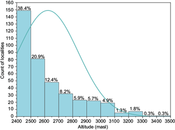
The region comprises 388 localities, including 362 rural communities and 26 urban areas across 31 municipalities. Seventeen of these municipalities are in Puebla, while the remaining 14 are in Veracruz. According to the 2020 locality-level census by INEGI (2020), the region’s total population is 333 465 inhabitants. According to CONAPO (2020), at least 83.5% of the localities (324) are classified as marginalized due to various types of deprivations. The most significant of these are related to basic housing and health services. Figure 1 displays the main features of the study area; additionally, Figure 2 displays the altitudinal distribution of the locations in 100-meter intervals.
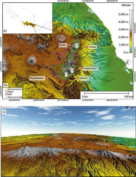
Fig. 1 Location of (a) the Neovolcanic Axis and (b) the study region with localities and automatic weather stations. (c) Oblique perspective from the coastline with the Mexican Central Plateau in the background and the center. Numbers correspond to the volcanoes Sierra Negra (1), Citlaltépetl (2), and Cofre de Perote (3).
2.2 Climatological data and processing
2.2.1 Tracking and monitoring of frontal systems, 2021-2022
In Mexico, the arrival of polar air masses begins in September and ends in May of the following year (CONAGUA, 2023). Therefore, tracking the advance of each of these air masses consisted of monitoring the day on which each cold front crossed the northern border of the country. From that moment on, it was tracked until the day that each frontal system associated with the cold air mass reached the center of the nation, as well as the day of its departure from the territory or its dissipation. The tracking was done through the Servicio Meteorológico Nacional (SMN; National Weather Service) webpage (https://smn.conagua.gob.mx/es/). Table I shows the date of entry into the study area and the days of affectation while the air mass remained in the area.
Table I Frontal systems that directly impacted the country during the winter of 2021-2022.
| Frontal system | Date of entry (north) | Arrival date (center) | Exit or disengagement | Hydrometeorological phenomena | Occurrence of snowfall per region of the country |
| 1 | September 21 | September 23 | September 26 | Rain | - |
| 2 | October 1 | October 5 | October 9 | Rain | - |
| 3 | October 10 | - | October 12 | Rain | - |
| 4 | October 13 | October 16 | October 19 | Rain | - |
| 5 | October 21 | - | October 23 | Rain | - |
| 6 | October 26 | October 27 | October 30 | Rain | - |
| 7 | November 3 | November 4 | November 7 | Rain | - |
| 8 | November 11 | November 13 | November 15 | Rain | - |
| 9 | November 18 | November 19 | November 21 | Rain | - |
| 10 | November 21 | November 22 | November 24 | Rain/SNWFL/SLT | N/NW |
| 11 | November 25 | November 25 | November 30 | Rain/SNWFL/SLT | N/NW |
| 12 | December 6 | - | December 8 | Rain/SNWFL/SLT | N/NW |
| 13 | December 10 | December 12 | December 13 | Rain/SNWFL/SLT | N/NW |
| 14 | December 14 | December 19 | December 23 | Rain/SNWFL/SLT | N/NW |
| 15 | - | - | - | - | - |
| 16 | December 25 | - | December 30 | Rain/SNWFL/SLT | N/NW |
| 17 | December 28 | - | December 31 | Rain/SNWFL/SLT | N/NW |
| 18 | December 31 | - | January 1 | Rain/SNWFL/SLT | N/NW |
| 19 | January 1 | January 2 | January 4 | Rain/SNWFL/SLT | C |
| 20 | January 5 | - | January 8 | Rain/SNWFL/SLT | C |
| 21 | January 8 | January 10 | January 13 | Rain/SNWFL/SLT | N/NW/C |
| 22 | January 14 | January 16 | January 17 | Rain/SNWFL/SLT | N/C |
| 23 | January 19 | January 21 | January 23 | Rain/SNWFL/SLT | N/NW/C |
| 24 | January 22 | January 25 | January 27 | Rain/SNWFL/SLT | N/NW/C |
| 25-26 | January 26 | January 28 | January 30 | Rain/SNWFL/SLT | N/NW/C |
| 27 | January 30 | - | - | Rain/SNWFL/SLT | N/NW/ |
| 28 | February 1 | February 3 | February 8 | Rain/SNWFL/SLT | N/NW/C |
| 29 | February 12 | February 13 | February 15 | Rain/SNWFL/SLT | N/NE/C |
| 30 | February 15 | February 18 | February 21 | Rain/SNWFL/SLT | NW/N |
| 31 | February 22 | February 27 | March 1 | Rain/SNWFL/SLT | NW/C |
| 32 | March 4 | - | March 5 | Rain/SNWFL/SLT | NW |
| 33 | March 5 | - | March 6 | Rain/SNWFL/SLT | NW |
| 34 | March 6 | March 8 | March 10 | Rain | - |
| 35 | March 11 | March 12 | March 13 | Rain/SNWFL/SLT | N/NW |
| 36 | March 14 | March 15 | March 16 | Rain | C? |
| 37 | March 17 | March 18 | March 20 | Rain | - |
| 38 | March 20 | March 22 | March 26 | Rain/SNWFL/SLT | N/NW |
| 39 | March 28 | - | April 2 | Rain/SNWFL/SLT | N/NW |
| 40 | April 2 | - | April 4 | Rain | - |
| 41 | April 6 | April 7 | April 8 | Rain | C? |
| 42 | April 12 | - | April 14 | Rain/SNWFL/SLT | NW? |
| 43 | April 18 | - | April 19 | Rain | C? |
| 44 | April 22 | - | April 24 | Rain | - |
| 45 | April 25 | - | abr-27 | Rain | - |
SNWFL: snowfall; SLT: sleet; N: north; NW: northwest; C: center; NE: northeast.
2.2.2 Analysis of air temperature and estimation of the lower limit for surface freezing
As with temporality concerning the monitoring of frontal systems, data for the same period were obtained from automatic meteorological stations (AMSs) located around and closer to the study region to monitor frontal systems. The stations store data every 10 min, providing a sufficiently complete data series from November 2021 to May 2022. The monthly data was downloaded from the official website of the SMN at https://smn.conagua.gob.mx/es/observando-el-tiempo/estaciones-meteorologicas-automaticas-ema-s. The data was tabulated based on the days each frontal system remained in the study region, from entry until departure or dissipation. This allowed observation of the thermal impact of each cold air mass that reached the area. A temperature graph was prepared for each AMS and front analyzed to aid interpretation. Table II displays the AMSs utilized for temperature analysis.
Table II Automatic meteorological (AMS) stations used for temperature analysis.
| AMS | Longitude (W) | Latitude (N) | Altitude (masl) | Average altitude (masl) |
| Perote | 97.26868 | 19.54516 | 2410 | 1718 |
| Xalapa | 96.90416 | 19.51250 | 1369 | |
| Coscomatepec | 97.04098 | 19.06602 | 1495 | |
| Tecamachalco | 97.72166 | 18.86638 | 2047 | |
| Orizaba | 97.09805 | 18.86527 | 1268 |
The study identified the time of greatest impact of each frontal system from the data series, based on the lowest temperature recorded at each meteorological station. The average altitude was calculated because of the different altitudes among the five AMSs (refer to Table II). Then, the air temperature vertical gradient (ATVG) was calculated for each event with the lowest temperature recorded. The gradient was obtained by the method applied by Soto et al. (2023a) and Soto and Cervantes (2023) through the use of a regression equation between the altitude and temperature variables:
where the intercept β 0 represents the magnitude of change of the temperature value with respect to the terrain elevation (Soto and Cervantes, 2023), that is, the ATVG of the area. According to the authors, calculating the ATVG for each time of lowest recorded temperature has the advantage of using more realistic conditions of vertical temperature variation for each specific occasion, as opposed to a standard monthly or seasonal gradient.
After obtaining the ATVG, the minimum temperature value for each meteorological station was adjusted to the average altitude previously calculated between the stations for each frontal system. The adjusted temperature was interpolated using the inverse distance weighted method (IDW), which is widely used and recommended by Soto and Delgado (2020) and Soto et al. (2023b) due to its ability to accurately represent the spatial distribution of temperature (Yuan et al., 2016). The temperature layer was interpolated to the average altitude, and a digital elevation model (DEM) of the study area was used to distribute the temperature values based on the variation in the height of the mountain range relief. To ensure modeling accuracy, a DEM with a spatial resolution of 15 m per pixel was used, obtained from INEGI (2013). The three-dimensional modeling was developed using Eq. (2):
where T
(x, y)
represents the relief-adjusted temperature value at a point (x, y) in the mountain range; T
az
is the zone average temperature for each frontal system;
From the temperature modeling, the lower altitudinal limit of air surface freezing (0 ºC isotherm) was extracted. The 0 ºC isotherm was used to determine the lower altitudinal limit of air surface freezing; from this, the polygon of the area that experienced freezing temperatures during each cold air mass was obtained. The number of localities and inhabitants exposed to freezing temperatures was also counted for each event based on their location within the corresponding polygon.
Finally, the daily cumulative precipitation reanalysis model GPM_3IMERGDL (Huffman et al., 2019) was used to identify possible snowfall occurrences in the region by overlaying the precipitation layer above the freezing surface. Using open-access satellite images (Landsat, Sentinel, Aster), depending on their availability, the presence of snow cover in the mountain range was corroborated. In cases where cloud cover did not obstruct the view, the presence of snow confirmed a snowfall occurrence. The snowpack’s extent was delimited, and its surface area was calculated. In cases where precipitation was present but not observable due to satellite temporal resolution or cloud cover, a possible but unconfirmed snowfall occurrence was considered based on thermal and precipitation conditions.
3. Results
The monitoring of frontal systems allowed us to obtain a total of 45 cold fronts (a very close value to the normal range) that had a complete evolution within the national territory and caused a decrease in temperature and/or precipitation, either solid (snow) or liquid, as well as those that had a displacement to the interior of the country. Table I chronologically shows each of these events and the weather conditions that prevailed according to the region affected.
Starting in May, warmer air from the equatorial region, both from the Pacific and the Caribbean, caused frontal systems that entered the country to become stationary and/or move eastward, reaching the waters of the Gulf of Mexico to dissipate without causing any continental effects.
3.1 Analysis of air temperature and estimation of the lower limit for surface freezing
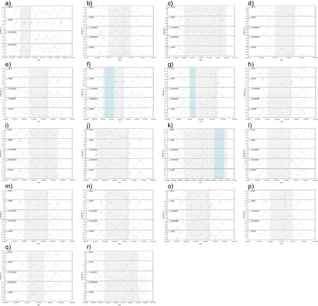
The study area was directly affected by 18 frontal systems, as shown in the temperature graphs sequence in Figure 3, which exhibits the decrease in temperature following the arrival of each cold front and throughout its duration. The affected days are indicated in light color. The lowest temperature reached in each event is indicated by the dotted line. The blue interval indicates the presence of confirmed snow, as seen in satellite images.
Based on the data provided, Table III was created to show the air temperature vertical gradients for each cold front, allowing the height of the 0 ºC isotherm to be estimated. At the same time, the calculated freezing area and the precipitation accumulated during the days of each frontal system can be noted. Additionally, snowfall occurrences have been recorded, both confirmed by satellite images and those not visually corroborated but considered possible based on temperature conditions and precipitation presence.
Table III Calculation of gradients and the lower limits of surface freezing for each frontal system that affected the study region. The extent of frozen surface, precipitation per affectation period, and the presence of snowfall are also reported.
| Automatic weather station | Altitude (masl) | Average altitude (masl) | Altitude Difference (m-1) | Temperature (ºC) | Regression equation | R2 | Temperature vertical gradient (ºC/m) | Altitude adjusted temperature (ºC) | Adjusted average temperature (ºC) | Altitude of 0ºC isotherm (masl) | Frozen area (km2) | Total accumulated precipitation (mm) | Snowfall null/possible/confirmed (date) |
| Cold front 11 | |||||||||||||
| Perote | 2410 | 1768 | -692 | 2.6 | y = -0.0076x + 20.096 | 0.84 | -0.0076 | 7.9 | 7.0 | 2644 | 1443.8 | 1.2 | Null |
| Xalapa | 1369 | 349 | 11.4 | 8.7 | |||||||||
| Coscomatepec | 1495 | 223 | 7.1 | 5.4 | |||||||||
| Tecamachalco | 2047 | -329 | 3.3 | 5.8 | |||||||||
| Orizaba | 1268 | 450 | ND | ND | |||||||||
| Cold front 13 | |||||||||||||
| Perote | 2410 | 1768 | -692 | 0.8 | y = -0.0114x + 28.518 | 0.95 | -0.0114 | 1.6 | 9.0 | 2502 | 2020.6 | 0 | Null |
| Xalapa | 1369 | 349 | 14.9 | 14.5 | |||||||||
| Coscomatepec | 1495 | 223 | 10.5 | 10.2 | |||||||||
| Tecamachalco | 2047 | -329 | 5.8 | 6.2 | |||||||||
| Orizaba | 1268 | 450 | 13.0 | 12.5 | |||||||||
| Cold front 14 | |||||||||||||
| Perote | 2410 | 1768 | -692 | -2.8 | y = -0.0103x + 23.27 | 0.95 | -0.0103 | 4.3 | 5.6 | 2259 | 2949 | 2.1 | Null |
| Xalapa | 1369 | 349 | 9.2 | 5.6 | |||||||||
| Coscomatepec | 1495 | 223 | 7.7 | 5.4 | |||||||||
| Tecamachalco | 2047 | -329 | 4.0 | 7.4 | |||||||||
| Orizaba | 1268 | 450 | 9.7 | 5.1 | |||||||||
| Cold front 16 | |||||||||||||
| Perote | 2410 | 1768 | -692 | 0.0 | y = -0.0067x + 16.254 | 0.97 | -0.0067 | 4.6 | 4.7 | 2426 | 2673.2 | 1.0 | Null |
| Xalapa | 1369 | 349 | 8.0 | 5.7 | |||||||||
| Coscomatepec | 1495 | 223 | 5.7 | 4.2 | |||||||||
| Tecamachalco | 2047 | -329 | 2.5 | 4.7 | |||||||||
| Orizaba | 1268 | 450 | 7.2 | 4.2 | |||||||||
| Cold front 19 | |||||||||||||
| Perote | 2410 | 1768 | -692 | 0.8 | y = -0.006x + 15.188 | 0.97 | -0.006 | 5.0 | 5.0 | 2531 | 1887.5 | 1.9 | Null |
| Xalapa | 1369 | 349 | 7.7 | 5.6 | |||||||||
| Coscomatepec | 1495 | 223 | 5.5 | 4.2 | |||||||||
| Tecamachalco | 2047 | -329 | 3.2 | 5.2 | |||||||||
| Orizaba | 1268 | 450 | 7.6 | 4.9 | |||||||||
| Cold front 21 | |||||||||||||
| Perote | 2410 | 1768 | -692 | 3.5 | y = -0.0065x + 18.471 | 0.94 | -0.0065 | 8.0 | 7.4 | 2842 | 916.3 | 33.3 | Confirmed Jan/10-11 |
| Xalapa | 1369 | 349 | 10.6 | 8.3 | |||||||||
| Coscomatepec | 1495 | 223 | 8.7 | 7.3 | |||||||||
| Tecamachalco | 2047 | -329 | 4.3 | 6.4 | |||||||||
| Orizaba | 1268 | 450 | 9.8 | 6.9 | |||||||||
| Cold front 22 | |||||||||||||
| Perote | 2410 | 1768 | -692 | 3.0 | y = -0.0045x + 13.929 | 0.90 | -0.0045 | 6.1 | 6.2 | 3095 | 498.2 | 8.8 | Confirmed Jan/16-17 |
| Xalapa | 1369 | 349 | 8.5 | 6.9 | |||||||||
| Coscomatepec | 1495 | 223 | 6.0 | 5.0 | |||||||||
| Tecamachalco | 2047 | -329 | 5.1 | 6.6 | |||||||||
| Orizaba | 1268 | 450 | 8.4 | 6.4 | |||||||||
| Cold front 23 | |||||||||||||
| Perote | 2410 | 1768 | -692 | 6.2 | y = -0.005x + 18.054 | 0.90 | -0.005 | 9.7 | 9.4 | 3610 | 199.4 | 14.3 | Possible above 4000 masl |
| Xalapa | 1369 | 349 | 12.5 | 10.8 | |||||||||
| Coscomatepec | 1495 | 223 | 9.9 | 8.8 | |||||||||
| Tecamachalco | 2047 | -329 | 7.4 | 9.0 | |||||||||
| Orizaba | 1268 | 450 | 11.1 | 8.9 | |||||||||
| Cold front 24 | |||||||||||||
| Perote | 2410 | 1768 | -692 | 3.4 | y = -0.0098x + 26.873 | 0.99 | -0.0098 | 10.2 | 10.1 | 2742 | 1167.6 | 0 | Null |
| Xalapa | 1369 | 349 | 14.0 | 10.6 | |||||||||
| Coscomatepec | 1495 | 223 | 12.3 | 10.1 | |||||||||
| Tecamachalco | 2047 | -329 | 6.8 | 10.0 | |||||||||
| Orizaba | 1268 | 450 | 14.1 | 9.7 | |||||||||
| Cold front 26 | |||||||||||||
| Perote | 2410 | 1768 | -692 | 0.5 | y = -0.0088x + 21.705 | 0.98 | -0.0088 | 6.6 | 6.5 | 2466 | 2292.6 | 1.6 | Confirmed Jan/28 |
| Xalapa | 1369 | 349 | 10.4 | 7.3 | |||||||||
| Coscomatepec | 1495 | 223 | 8.7 | 6.7 | |||||||||
| Tecamachalco | 2047 | -329 | 3.3 | 6.2 | |||||||||
| Orizaba | 1268 | 450 | 9.7 | 5.7 | |||||||||
| Cold front 28 | |||||||||||||
| Perote | 2410 | 1768 | -692 | 4.0 | y = -0.0025x + 9.5589 | 0.73 | -0.0025 | 5.7 | 5.3 | 3824 | 109.1 | 5.0 | Feb/8-9 |
| Xalapa | 1369 | 349 | 7.0 | 6.1 | |||||||||
| Coscomatepec | 1495 | 223 | 4.8 | 4.2 | |||||||||
| Tecamachalco | 2047 | -329 | 4.0 | 4.8 | |||||||||
| Orizaba | 1268 | 450 | 6.6 | 5.5 | |||||||||
| Cold front 29 | |||||||||||||
| Perote | 2410 | 1768 | -692 | -0.7 | y = -0.008x + 18.959 | 0.99 | -0.008 | 4.8 | 5.2 | 2370 | 2949 | 1.1 | Possible |
| Xalapa | 1369 | 349 | ND | ND | |||||||||
| Coscomatepec | 1495 | 223 | 6.8 | 5.0 | |||||||||
| Tecamachalco | 2047 | -329 | 3.3 | 5.9 | |||||||||
| Orizaba | 1268 | 450 | 8.8 | 5.2 | |||||||||
| Cold front 30 | |||||||||||||
| Perote | 2410 | 1768 | -692 | 3.5 | y = -0.0066x + 19.036 | 0.88 | -0.0066 | 8.1 | 7.6 | 2884 | 824.4 | 0.7 | Possible |
| Xalapa | 1369 | 349 | 11.7 | 9.4 | |||||||||
| Coscomatepec | 1495 | 223 | 9.1 | 7.6 | |||||||||
| Tecamachalco | 2047 | -329 | 4.5 | 6.7 | |||||||||
| Orizaba | 1268 | 450 | 9.3 | 6.3 | |||||||||
| Cold front 31 | |||||||||||||
| Perote | 2410 | 1768 | -692 | -1.7 | y = -0.0081x + 18.658 | 0.89 | -0.0081 | 3.9 | 4.7 | 2303 | 2949 | 0 | Null |
| Xalapa | 1369 | 349 | 9.1 | 6.3 | |||||||||
| Coscomatepec | 1495 | 223 | 4.9 | 3.1 | |||||||||
| Tecamachalco | 2047 | -329 | 3.5 | 6.2 | |||||||||
| Orizaba | 1268 | 450 | 7.8 | 4.2 | |||||||||
| Cold front 34 | |||||||||||||
| Perote | 2410 | 1768 | -692 | 8.1 | y = -0.0049x + 18.925 | 0.78 | -0.0049 | 11.5 | 11.3 | 3862 | 97.1 | 0 | Null |
| Xalapa | 1369 | 349 | 16.5 | 14.8 | |||||||||
| Coscomatepec | 1495 | 223 | 10.4 | 9.3 | |||||||||
| Tecamachalco | 2047 | -329 | 7.7 | 9.3 | |||||||||
| Orizaba | 1268 | 450 | 14.0 | 11.8 | |||||||||
| Cold front 35 | |||||||||||||
| Perote | 2410 | 1768 | -692 | 0.9 | y = -0.0058x + 15.844 | 0.87 | -0.0058 | 4.9 | 5.9 | 2732 | 1197.9 | 0.3 | Null |
| Xalapa | 1369 | 349 | 8.1 | 6.1 | |||||||||
| Coscomatepec | 1495 | 223 | 6.1 | 4.8 | |||||||||
| Tecamachalco | 2047 | -329 | 5.6 | 7.5 | |||||||||
| Orizaba | 1268 | 450 | 8.6 | 6.0 | |||||||||
| Cold front 36 | |||||||||||||
| Perote | 2410 | 1768 | -692 | 4.3 | y = -0.0076x + 23.707 | 0.81 | -0.0076 | 9.6 | 10.6 | 3119 | 474.7 | 0 | Null |
| Xalapa | 1369 | 349 | 15.5 | 12.8 | |||||||||
| Coscomatepec | 1495 | 223 | 108 | 9.1 | |||||||||
| Tecamachalco | 2047 | -329 | 9.8 | 12.3 | |||||||||
| Orizaba | 1268 | 450 | 12.7 | 9.3 | |||||||||
| Cold front 38 | |||||||||||||
| Perote | 2410 | 1768 | -692 | -0.6 | y = -0.0064x + 16.118 | 0.82 | -0.0064 | 3.8 | 5.2 | 2518 | 1960.2 | 0 | Null |
| Xalapa | 1369 | 349 | ND | ND | |||||||||
| Coscomatepec | 1495 | 223 | 5.9 | 4.5 | |||||||||
| Tecamachalco | 2047 | -329 | 5.3 | 7.4 | |||||||||
| Orizaba | 1268 | 450 | 7.9 | 5.0 | |||||||||
The resulting maps in Figure 4 display the modeling of surface temperature for each of the cold fronts, based on the gradients in Table III. The 18 maps are presented chronologically according to the date of occurrence of freezing, corresponding to the frontal systems that affected the study region.
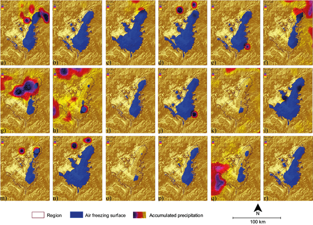
The surface and distribution of the areas affected by freezing according to each cold front that arrived in the region are shown in blue in Table III and Figure 4. On at least three occasions, the entire surface of the study area (2949 km2) was under freezing conditions (Fig. 4c, l, n); at the same time, the presence of precipitation coinciding with temperatures below 0 ºC can be noted, implying the potential possibility of snowfalls, some of which have been confirmed by remote sensing. Figure 5 shows three episodes of snowfall occurrence observed using RGB imagery from the Sentinel 2 satellite:
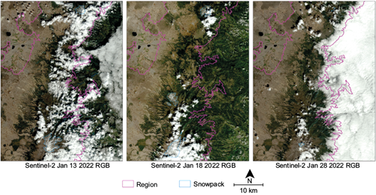
Fig. 5 Sentinel 2 RGB images showing snow accumulation (blue polygons). From left to right, frontal systems 21 (January 8-13), 22 (January 14-17), and 26 (January 26-30).
Table III shows that at least three snowfalls were confirmed: the first one on January 13, 2022, with a snow cover area of 32.5 km2; the second one on January 18, 2022, with an area of 46.7 km2; and the third one on January 28, 2022, covering 2.2 km2. However, the cloudy conditions prevented snowpack observation during the days that suggested snow precipitation due to temperature conditions and precipitation. It is worth noting that the snow covered the upper parts and lower slopes of Pico de Orizaba, Sierra Negra, and Cofre de Perote in all three cases. Even more, during the snowfall on January 18, the snow covered not only the peaks but also a central part of the mountain range.
The graphs in Figure 6 show the total number of villages, both rural and urban, that were exposed to freezing temperatures, as well as the number of people who were exposed or could have been affected. The corresponding graph differentiates between localities and inhabitants according to the states to which they belong.
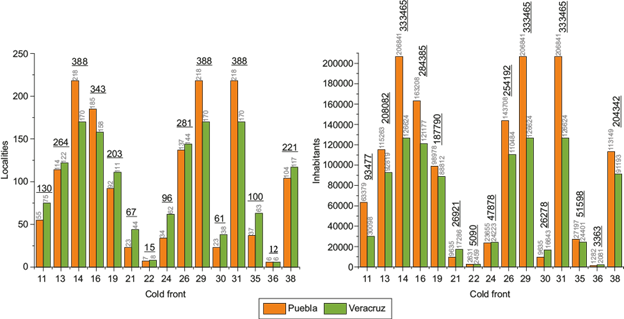
Fig. 6 Number of localities and inhabitants exposed to freezing temperatures per cold front and state. The underlined numbers represent the sum of the two states for each of the frontal systems.
The state of Puebla has a greater number of localities and inhabitants than Veracruz because the former has 17 municipalities in the region, while the latter only 14. As a result, Puebla has a total of 218 villages, while Veracruz has 170. During frontal systems 14, 29, and 31, freezing temperatures affected all 388 localities in the region and their 333 465 inhabitants, as depicted in the maps in Figure 4. The number of localities and the number of inhabitants affected varies according to the altitude at which the 0 ºC isotherm was ubicated in each of the cold fronts (see Table III); therefore, it ranges from 2259 masl (covering the entire study region) to 3862 masl, with a direct impact on the localities within each altitudinal range at which the freezing isotherm was located.
4. Discussion
4.1 Climatic conditions
The recent changes in climate conditions, specifically air temperature, over the last few decades have caused a decrease in the velocity of the jet stream. As a result, the boreal polar cell has extended to latitudes well below its average limits, leading to an increase in the number of winter storms that now cover the entire US territory. These storms have also caused collateral effects in the Mexican territory, which is why the findings of this work partially confirm the increasingly severe impacts of winter weather in the northern hemisphere over time, as previously noted by Pons et al. (2016) and Quante et al. (2021).
The winter of 2021-2022 in Mexico was one of the most intense in terms of temperature drops, frost, and snowfall. The climatological statistics for the country show that during the 2021-2022 winter season, frontal systems arrived and evolved within the national territory at a rate similar to the average. However, some of these cold fronts had direct implications for temperature and precipitation in the northern states and mountainous areas of the country’s center, resulting in freezing environmental conditions and occasional snowfall.
The study region was directly affected by 18 of the total number of frontal systems that entered Mexican territory, as the altitude of the region’s relief (between 2400 and 5610 masl) determined the presence of freezing temperatures during the arrival of these cold fronts; this is why the total surface of the region (2949 km2) remained frozen in at least three of the 18 cold fronts that affected it. In the rest of the occasions, the freezing isotherm altitude was located according to the temperature variation with respect to the terrain (i.e., between 2259 and 3862 masl), as seen in Figure 4. However, for a more detailed understanding of the temperature ranges during each cold front, especially regarding freezing temperatures and specific locations, refer to the graphical representation in Figure 7.
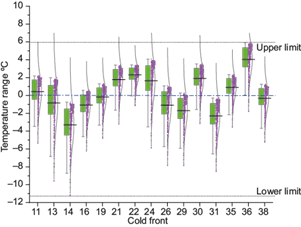
The extreme temperature values recorded in the localities of the study region (pink dots) can be observed, ranging from ~6 to just under -11 ºC (dashed gray lines). The highest temperatures correspond to the localities in the area’s lower parts, while those at higher altitudes recorded the lowest temperatures. According to Figure 7, the concentration of settlements is directly related to their altitude; therefore, most settlements are located at the top of the boxes (lower altitude: 2400 masl). On the other hand, higher and more isolated localities show greater dispersion compared to the average (highest altitude locality: 3404 masl), as seen in Figure 2.
The variation of the ATVG between one cold front and another (in this case, from -0.0025 to -0.0114 ºC per meter of elevation of the relief) emphasizes the need to calculate a specific ATVG for each study area and for each time that it is necessary to estimate the temperature in mountain relief, just as Soto and Delgado (2020) indicate. This is calculated through the values recorded by the stations surrounding the area of interest, as done in this work. Otherwise, using a standard ATVG, whether global, annual, or seasonal, would generate a high degree of uncertainty when calculating the temperature in mountainous areas for a specific occasion.
During cold front 14, the region experienced a significant drop in temperature. The city of Perote, which typically has an annual maximum temperature of 21.7 ºC and a minimum of 3.8 ºC, reached a low of -2.8 ºC. This temperature decrease is comparable to the average temperature observed throughout the year in the lower zone of the Pico de Orizaba glacier, which is located at 5130 masl (Soto et al., 2019). Satellite images were used to confirm the correlation between the freezing temperature and precipitation patterns in the region. The images display layers of snow covering the summits, slopes of the three main mountains, and part of the central zone of the mountain range. Given the thermal conditions and humidity, it is likely that there was a short duration of snow or sleet precipitation; however, due to the temporal resolution of the satellite images and the presence of cloudiness, it cannot be confirmed.
Environmental impacts resulting from the displacement of polar air masses in North America are becoming more frequent and intense. For instance, in the second week of January 2024, severe winter storms hit vast regions of the US, causing temperatures to drop by up to ~10 ºC below the seasonal average and resulting in 83 confirmed deaths (Gorman, 2024). In Mexico, temporary road closures in northern states have been caused by frontal systems 27 and 28, which brought snowfall. Also, low temperatures and humidity caused snowfall at elevations above ~4000 masl in the main mountains of the Neovolcanic Axis. In Veracruz, the highlands experienced a temperature of -10 ºC (Vázquez, 2024) and received intense precipitation that covered the summits and slopes of the Sierra Negra, Pico de Orizaba, and Cofre de Perote volcanoes with snow (Reyes, 2024).
Although only one year of the winter season has been studied, this research aims not to compare it with the climatological conditions of previous years. Instead, the objective is to highlight how the 2021-2022 winter impacted a region of high social, economic, and ecosystemic value. However, this temporality can also cause bias if a statistical climatological analysis is intended. For this reason, and to mitigate as much as possible the potential limitation of this study, it is recommended that the winter seasons in the region be monitored continuously to obtain higher-quality data for subsequent works, where more specific impacts can be analyzed, such as the generation of droughts and the decrease in agricultural production, among other important consequences.
Regardless of all the above, and from a climatological perspective, the procedures developed in this work have demonstrated the accuracy of the methodology used to analyze the impact of winter cold conditions. This methodology can be applied not only in the study region but also in other mountainous areas throughout the country, such as the Iztaccíhuatl-Popocatépetl strip, the mountainous regions of Chihuahua and Durango, as well as Baja California, among other areas commonly affected by severe winter cold. At the same time, it helps to understand the potential impact of freezing environments on ecosystems and, more importantly, on human settlements located within these regions.
4.2 Impact on the region’s population
Of the 388 localities in the study region, which includes both Puebla and Veracruz, with a total population of 333 465, many experienced freezing conditions during the winter of 2021-2022. The severity of the temperature drop varied depending on altitude. Frontal systems 14, 16, 29, and 31 placed almost the entire population under negative temperatures. However, frontal systems 22 and 36 had the least impact on inhabitants, affecting only those in localities at higher elevations. This is because some settlements are located in the highest parts of the mountain range (>3000 masl). Nevertheless, these two cold fronts affected at least 5090 and 3363 inhabitants of these localities, respectively.
The magnitude of the impact on the population’s health depends mainly on their level of vulnerability to intense cold conditions, which is commonly associated with the degree of marginalization of the localities. According to data from CONAPO (2020), it is possible to categorize the different degrees of marginalization of urban and rural localities in the study region. It is important to note that, according to INEGI (2021), the main difference between urban and rural settlements is based on whether the former has a population greater than 2500 inhabitants. Table IV shows the number of urban and rural localities and their respective populations according to their levels of marginalization.
Table IV Levels of marginalization per state.
| Level of marginalization | Puebla | Veracruz | ||
| Number of localities | Total population | Number of localities | Total population | |
| Very high | U/R: 0/6 | 310 | U/R: 0/6 | 526 |
| High | U/R: 1/28 | 12 330 | U/R: 2/62 | 22 579 |
| Medium | U/R: 10/71 | 64 423 | U/R: 6/51 | 34 779 |
| Low | U/R: 16/33 | 126 712 | U/R: 7/11 | 68 585 |
| Very low | U/R: 0/11 | 2611 | U/R: 0/3 | 47 |
U: urban localities; R: rural localities.
Of all the communities in the study region, localities in Veracruz with high (43.2%) and medium (38.5%) degrees of marginalization are prevalent, while in Puebla those with medium (46.0%) and low (27.8%) degrees of marginalization are more common. However, most of the population in both states resides in the low category, which is due to the presence of densely populated urban areas that offer more basic services. However, the most vulnerable populations are those lacking basic services due to their remote location, which may increase their vulnerability to the intense cold of winter. In the mountainous regions of Mexico, this largely marginalized population is frequently located at altitudes above 2500 masl; the statement is congruent with the remote human settlements within the Pico de Orizaba-Cofre de Perote mountain range.
During the winter of 2021-2022, 13 of the 15 frontal systems that impacted the study region had continuous effects on 11 remote rural localities, which had a combined population of 3359 inhabitants. These areas are notable for their high (eight localities) and medium (three localities) levels of marginalization, which likely impact their ability to cope with adverse weather conditions, particularly freezing temperatures. If we consider future projection models, which indicate an increase in severe cold conditions occurring with greater frequency and intensity, this region’s inhabitants will need to increase their capacity to adapt to the coming scenarios.
Another topic worth addressing is the attraction that snow causes for people unfamiliar with this element. It is common for residents of nearby cities to visit snowy areas for recreational purposes, often without considering the potential health risks posed by low temperatures. This situation calls for implementing community-level preventive measures to avoid cold-related illnesses.
5. Conclusions
The changing global climate conditions are causing a wider range of extreme temperature values, among other consequences. In recent years, the northern hemisphere has experienced a higher frequency of severe winter storms that have paralyzed all kinds of daily activities and, in extreme cases, have claimed the lives of many people. The region between Pico de Orizaba and Cofre de Perote frequently experiences freezing conditions during winter. Due to social marginalization, low temperatures have a greater impact on the most vulnerable population. However, among all the locations within the study region, those corresponding to the state of Veracruz appear to be the most susceptible to these impacts due to their higher vulnerability.
The contributions of this work can be differentiated from two points of view. The first proposes a methodology useful for estimating temperature conditions prevailing in high mountain environments where the lack of climatological stations is common. Therefore, the methods used in this work can be applied to other regions and any period of interest. The second contribution relates to the harsh winter conditions that the most marginalized mountain populations may be exposed to, which can represent a greater vulnerability to the harshness of severe winter weather. It is important to remember that three-quarters of the Mexican territory is composed of mountainous relief, and a large number of populations are located in high-altitude areas. This situation invites reflection on the future scenarios that these populations will face in the extreme conditions of a changing climate. Simultaneously, this partially highlights the necessity for local disaster risk management in circumstances of low temperatures.

