2.Problem formulation

2.1.Physical model

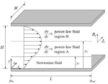
The present work analyzes the transport of two immiscible fluids in a parallel flat plate microchannel of height H, width W and length L, as shown in Fig.1. The Cartesian coordinate system (x,y,z) is located at the bottom of the channel inlet. Fluid pumping primarily occurs through MHD effects; however, a pressure differential can be generated between the inlet and outlet of the microchannel (Δp=pout-pin), producing a common constant pressure gradient over fluid layers. The flow field is made up of two layers of fluids divided by the interface position y₁. For the range of 0<y<y1, there is a Newtonian fluid (driven fluid), while for the range of y1<y<H, there is a non-Newtonian fluid (driving fluid) composed of a mixture of an ionized solution and a solute which behaves like a power-law fluid. Here, B_y on the y-axis is the magnetic field from permanent magnets located at the upper and bottom walls of the microchannel, and J_z on the z-axis is the electric current density generated by an electric field from a pair of electrodes placed at the lateral walls; these interact transversally to each other to produce the Lorentz forces that act on the electrically conducting non-Newtonian fluid, resulting in dragging of the electrically non-conducting Newtonian fluid by viscous forces. On the other hand, the power-law fluid layer can be divided into two regions A and B, showing the velocity gradient behavior regarding the increase (du/dy>0) and decrease (du/dy<0) of the velocity profile slope. The distance y₂ as a fictitious interface indicates the point at which the maximum velocity of the non-Newtonian fluid is reached.

Figure 1 Sketch of the magnetohydrodynamic flow in a parallel flat plate microchannel. 

2.2.General governing equations

The governing equations for incompressible fluids that describe the flow field are given by the continuity equation

and the Cauchy momentum equation

where v is the velocity vector, ρ is the fluid density, t is the time, p is the pressure, τ is the stress tensor, and F is the body force vector. Here, body forces appear due to the application of the electric and magnetic fields; their magnitude is determined by

where J represents the electric current density given by Ohm’s law as J=σ(E+V×B); σ denotes the electric conductivity, and E and B are the electric and magnetic field vectors, respectively. On the other hand, the generalized constitutive equation for the power-law fluid is expressed as

where η is the dynamic viscosity and γ̇ is the rate-of-strain tensor defined as γ̇=∇v+(∇v)T. Furthermore, the viscosity for fluids that follow a behavior based on the rheological power-law model is

where m is the flow consistency coefficient and n is the flow behavior index. In the case of a Newtonian fluid with constant viscosity μ, from Eq. (4), ηγ̇=μ.

2.3.Simplified mathematical model

The mathematical model used to solve the MHD flow can be simplified by taking into account the following considerations: i) Steady, laminar and fully developed flow is assumed ^5,12,14,34. ii) The electrical and physical properties of fluids are assumed to be constant ^{32 44 45}. iii) Laminar flow is assumed for low Reynolds number, i.e., Re(=ρHuc/η)=O(1) or less, where uc is the characteristic flow velocity. iv) The densities of fluids can be considered equal or matched; thus, the gravitational effects are neglected (30)(31),(36) . v) The microchannel is long enough in relation to its height, i.e., L≫H, to use lubrication theory and neglect the end effects ⁴⁷. vi) An infinite extent of the flow domain is assumed along the z-axis, i.e., W≫H, to disregard any effects of the sidewalls and secondary flows . vii) In MHD micropumps, induced magnetic fields due to the fluid motion are extremely weak and can be disregarded ^18,48. viii) By maintaining the electric potential across the electrodes in contact with the aqueous solution within a few mV around the standard equilibrium voltage of 1.23 V ^8,18,49 and establishing an electric current between electrodes of less than 0.1 mA ⁵⁰, the bubble formation by electrolysis can be neglected. To evaluate the orders of magnitude presented in this paragraph and throughout this work, see the physical and geometric parameters presented in Sec. 4.

With the assumptions mentioned above, a unidirectional flow and a planar liquid-liquid interface between the fluids can be considered. Specifically for the conducting fluid, the well-known Hartmann flow is recovered ^3,18,47. Therefore, the governing equations given by Eqs. (1) and (2) are simplified in Cartesian coordinates for the Newtonian fluid as

and for the non-Newtonian fluid as

where u1=u1(y) and u2=u2(y) are the fluid velocities, E_z is the electric field on the z-axis, and the pressure gradient, provided by a syringe pump, is defined as dp/dx=px=(pout-pin)/L.

2.4.Boundary conditions

To solve the flow field established by Eqs. (6) and (7), the following boundary conditions are presented depending on the type of interface, beginning with the no-slip boundary conditions on the walls located at the upper and lower solid-liquid interfaces of the channel, that is,

and

For the liquid-liquid interface at y = y₁, the velocity continuity condition is considered as follows:

together with the shear stress balance condition

2.5.Dimensionless mathematical model

To normalize the mathematical model that describes the MHD flow behavior, the following dimensionless variables are introduced:

where the characteristic velocity is defined by uc=σrefEzByH2/ηref ⁴⁸; the subscript “ref” indicates a reference condition for aqueous electrolyte solutions with T_ref = 298.15 K ^51-55. Hence, the momentum conservation equations described in Eqs. (6) and (7) can be written in dimensionless form as

and

where the dimensionless parameters that appear are

where Γ is the ratio of pressure to magnetic forces, while μ¯ and η¯ represent the viscosity ratios of the Newtonian and non-Newtonian fluid, respectively. As a reference for this work, consider px∼σEzBy ^11,48, whose sign depends on whether the pressure gradient favors or adversely affects the flow. Therefore, Γ∼±σ/σref. On the other hand, Ha is the Hartmann number and indicates the relationship between the magnetic forces and the viscous forces, and Ω* is the load parameter. Here, η∼muc/Hn-1 represents the order of magnitude of the non-Newtonian fluid viscosity. The parameter Ω*Ha2=uc,2/uc indicates the ratio of magnetic effects acting on a power-law fluid compared with the influence on a reference Newtonian fluid, where uc,2∼σEzByH2/η. Derived from the physical and geometric conditions of the microchannel system in this work, the following orders of magnitude are considered: Γ=O(1), μ¯=O(1), η¯=O(1), Ha≪1, Ω*≫1 and 0≤Ω*Ha2≤100.

Following the same procedure to obtain the dimensionless expressions of the boundary conditions, which consists of substituting Eq. (12) into Eqs. (8)-(11), the following results were achieved. For the solid-liquid interfaces, the no-slip conditions on the walls of the microchannel are

and

For the liquid-liquid interface at y¯=y¯1, the velocity continuity condition is

together with the shear stress balance condition

3.1.Velocity profile for the Newtonian fluid

For the Newtonian fluid, the velocity profile is quickly found by integrating Eq. (13) twice with respect to the transverse coordinate y¯, yielding

where C₁ and C₂ are integration constants.

3.2.Velocity profile for the power-law fluid

To obtain the velocity profile of the non-Newtonian fluid layer, first, the Hartmann number is assumed to be very small, i.e., Ha≪1, due to the microchannel scale and the type of buffer solution ^18,56, causing the third term on the right-hand side of Eq. (14), known as the Hartmann breaking term, to be neglected, yielding

Then, integrating once with respect to the transverse coordinate y¯, in Eq. (21) results in

where C₃ is an integration constant, and λ=(-Γ+Ω*Ha2)/η¯, which may be positive or negative. On the other hand, when the velocity profile of the power-law fluid has a maximum or minimum in the range y¯1≤y¯≤1, the non-Newtonian fluid has two regions corresponding to positive and negative signs for the velocity gradient, being positive for region-A and negative for region-B (see Fig. 1), a circumstance that must be considered within the absolute value of Eq. (22) ^57,58. Equation (22) for each case is then rewritten as follows:

and

where C_3,A and C_3,B are the corresponding integration constants for region-A and region-B, respectively. Hence, Eqs.(23) and (24) can be simplified as follows:

and

where s = 1/n, and to avoid any singularity with the λ sign in the process, λs=λ|λ|s-1 ⁵⁸. Finally, the velocity profile for each section is obtained by integrating Eqs. (25) and (26), yielding the following expressions:

and

where C_4,A and C_4,B are integration constants.

3.3.Application of boundary conditions at real interfaces

To find the integration constants C1,C2,C3 and C₄ of the velocity profiles given in Eqs. (20), (37) and (38), the boundary conditions given by Eqs. (16)-(19) must be applied. First, Eq. (16) is substituted into Eq. (38) at y¯=1, yielding

Second, Eq. (17) is substituted into Eq. (20) at y¯=0, resulting in

Third, Eqs. (20) and (37) are substituted into Eq. (18) at y¯=y¯1, yielding the following expression:

Fourth, Eqs. (20) and (23) are substituted into Eq. (19) at y¯=y¯1, where it is considered that C3,A=C3, yielding

To find the constants C₁, C₃ and C₄, the Newton-Raphson method is used to solve the system of non-linear equations formed by Eqs. (39), (41) and (42); here, the convergence criterion is 10^-6, and the proposed initial value is 1.

3.4.Flow rate

The total dimensionless flow rate is determined by integrating the velocity profile of each fluid layer with respect to the transverse coordinate y¯, which means that

Here, Q¯1 represents the flow rate of the Newtonian fluid, which is defined as

while Q¯2 corresponds to the flow rate of the non-Newtonian fluid, given by

Solving the integrals and taking into account that C₂ = 2 and y¯2=C3 leads to

and

Finally, a mathematical expression for the total flow rate is found by substituting Eqs. (46) and (47) into Eq. (43), leading to

where the dimensionless variable for this process is Q¯=Q/Qc; Qc=ucH represents the characteristic flow rate. All aforementioned values are per unit of the channel width.

4.1.Velocity field

In Fig. 2, the transport of two immiscible fluids driven by purely MHD forces is analyzed. Figure 2a) presents the velocity profile as a function of the dimensionless transverse coordinate y¯, as well as the combination of the dimensionless parameters shown in the graph. The liquid-liquid interface position y¯1=0.2 indicates the spatial distribution of each fluid layer in the channel, where it can be observed that most of the space corresponds to the non-Newtonian fluid layer. Furthermore, considering that the Newtonian fluid is electrically non-conducting, the magnitude of the velocity profile depends mainly on the electrical properties of the power-law fluid, while the Newtonian fluid moves due to viscous drag effects. In this graph, the results are based on different values of the flow behavior index 𝑛 in the range of 0.5≤n≤1.5. Shear-thickening fluids (also called dilatant fluids) are obtained for values of n > 1, while shear-thinning fluids (also called pseudoplastic fluids) result for n < 1, and when n = 1, the case of a Newtonian fluid is recovered. Taking into account that the viscosity η¯ is a function of the rate-of-strain tensor γ̇ (see Eq. (5)), the highest velocity is achieved when n = 0.5 due to the fact that for a shear-thinning fluid, an increase in the shear rate will reduce the viscosity ⁵⁷, also causing fluid conduction to improve. The opposite effect occurs for a shear-thickening fluid, i.e., the lowest velocity is reached when n = 1.5 . Although the velocity increase is more pronounced in the central region of the power-law fluids, a significant difference is shown between the velocity profiles. This difference tends to diminish when approaching the liquid-liquid and solid-liquid interfaces due to the viscous drag resistance and the no-slip boundary condition, respectively. It is clear that the use of shear-thinning fluids increases the velocity of the non-conducting Newtonian fluid. On the other hand, the point y¯2 where the maximum velocity is located in the non-Newtonian fluid layer, moves away from the liquid-liquid interface position y¯1 when the value of the flow behavior index n decreases. Correspondingly, in Fig. 2b), the shear stress distribution as a function of the transverse coordinate y¯ is shown, for the same combination of dimensionless parameters as in Fig. 2a). The generalized relationship for the dimensionless shear stress for any fluid in the present investigation is obtained from Eq. (4) as

where τ¯xy=τxyH/ηrefuc. Therefore, the shear stress for the non-Newtonian fluid is determined from Eq. (49) and with the aid of Eq. (22), yielding the expression τ¯xy,2=-η¯λ(C3-y¯) in the range of y¯1≤y¯≤1. In the case of the Newtonian fluid, the shear stress is determined from Eq.(49) together with Eq.(20), and by considering that n = 1 and η¯=μ¯, obtaining the relationship of τ¯xy,1=-Γy¯-μ¯C1 applied at 0≤y¯≤y¯1. As can be seen in Fog. 2b), the greatest shear stresses are located at the extreme limits of the driving non-Newtonian fluid, i.e., at the liquid-liquid interface placed at y¯=y¯1 and the solid-liquid interface placed at y¯=1, locations where the fluid offers the highest flow resistance. In this context, the non-Newtonian fluid offers the lowest resistance to flow when τ¯xy,2=0 at the positions y¯2=0.5764,0.5456,0.5200,0.5006, and 0.4861 for n = 0.5,0.75,1,1.25 and 1.5, respectively. The aforementioned finding indicates that the slope or velocity gradient at these positions is du2/dy=0 (see Fig. 2a) for how the velocity profile reaches the maximum velocity and the change in sign of the velocity gradient occurs for the rheological power-law model), which occurs when y¯2=C3. In the case of the Newtonian fluid that lies between the limits y¯=0 and y¯=y¯1, both the shear stress and the velocity gradient remain constant (see F2a) for the slanted velocity profile).

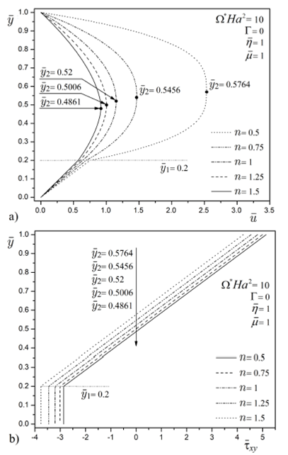
Figure 2 Dimensionless a) velocity profile and b) shear stress distribution for a purely MHD flow for different values of the flow behavior index n. 

Figure 3 shows an increase in the velocity profile due to an increment in the magnetic effects applied to the power-law fluid; compared to the influence on a reference Newtonian fluid, this behavior is reflected by the parameter Ω*Ha2, which is sensitive to the reference conditions. For this case, the flow behavior index is n = 1.4, describing a shear-thickening fluid. Furthermore, it can be seen that the magnetic effects act on transverse coordinate y¯, which creates the parabolic shape in the flow field of the power-law fluid. This result is possible when the Hartmann number is assumed to be very small, i.e., Ha≪1, since in this limit, the Hartmann breaking term is neglected. However, when the velocity profile reaches the liquid-liquid interface at y¯=y¯1, it exhibits a linear behavior since the Newtonian fluid is not an electric conductor, and its displacement is due to the viscous drag effect. Additionally, it is shown that the velocity of the non-conducting Newtonian fluid increases significantly with the parameter Ω*Ha2 compared with the previous 2 where Ω*Ha2=10 was used.

Figure 3 Dimensionless velocity profile for a purely MHD flow for different values of Ω*Ha2. 

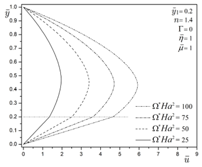
Figure 4 analyzes the velocity field of the viscous micropump under combined MHD and pressure-driven effects; here, three values of parameter Γ (=-2,0,2) and two values of the dynamic viscosity of the non-conducting Newtonian fluid μ¯(=0.7,1) are used. The pumped fluid is a shear-thinning fluid with n = 0.8. The pressure gradient values depend on the pressure exerted at the inlet and outlet of the channel, which is generated with a syringe pump. Under this scheme, the positive values are reached when pout-pin>0 and negative values result when pout-pin<0, while for pout-pin=0 the pressure gradient effects are considered null and the purely magnetohydrodynamic flow is consequently recovered. For the first case Γ = 2, the pressure at the outlet is higher than that at the channel inlet, which means that the pressure gradient is applied in the negative direction of the x-axis, opposing the Lorentz forces; as a result, the lowest velocity profiles in magnitude are obtained. This behavior is shown by the solid lines, where it is observed that the power-law fluid moves in the same direction as the flow, and the Newtonian fluid moves opposite to the flow because it is only affected by pressure forces. For the second case Γ = 0, the only driving forces are the magnetic effects exerted by the parameter Ω*Ha2=5. For the third case Γ = -2 , the pressure at the inlet is higher than that at the channel outlet, the pressure forces are in the same direction as the flow, and consequently, greater magnitude velocity profiles are achieved. The linear velocity profile of the Newtonian fluid is lost when the pressure gradient is imposed, i.e., when Γ = -2 and Γ = 2. Additionally, the viscosity parameter turns out to be relevant in fluid conduction since it is responsible for regulating the resistance to movement offered by the fluid layer. For de above, by decreasing the viscosity ratio μ¯=1 (lines without symbols) to μ¯=0.7 (lines with symbols), the Newtonian fluid pumping is increased in favor of or against the flow, and the pressure gradient effects magnify this situation.

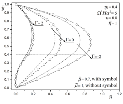
Figure 4 Dimensionless velocity profile for the combined MHD and pressure-driven flow for different values of Γ and μ¯. 

The purely MHD flow is shown in Fig. 5. As previously mentioned, shear-thinning fluids have better conduction than shear-thickening fluids. The aforementioned is reflectedby the magnitude difference between lines with symbols for n = 0.6 compared to lines without symbols for n = 1.2. On the other hand, the flow resistance imposed by the power-law fluid is represented by the viscosity ratio η¯ in the range of 0.7 to 1.3, which means that the flow resistance is lower for values less than unity, which is transmitted as better conduction of the Newtonian fluid. In comparison, for values greater than unity, the flow resistance increases, and lower conduction of the Newtonian fluid is consequently presented. Finally, η¯=1 indicates that the viscosity of the reference Newtonian fluid is reached. In this sense, the highest velocity magnitudes are achieved when the viscosity offers less resistance to flow, which is achieved with η¯=0.7.

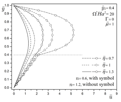
Figure 5 Dimensionless velocity profile for a purely MHD flow for different values of the viscosity ratio η¯ and flow behavior index n. 

Figure 6 represents the micropump flow field formed by two layers of immiscible fluids, where, as in the previous figures, the power-law fluid works as a driving fluid and the Newtonian fluid as a driven fluid. Here, two cases corresponding to the driving fluid are presented, the first for a shear-thinning fluid of n = 0.75 and the second for a shear-thickening fluid of n = 1.25. In addition to this, three liquid-liquid interface positions (given by y¯1=0.25,0.5,0.75) that modify the thickness of each fluid layer are established. These interface positions y¯1 are selected to analyze the behavior of the flow field, taking into account the following situations when the thickness of the non-conducting fluid is less than, equal to or greater than the thickness of the conducting fluid. However, the number of possible combinations is not limited to only these three values. As can be seen, when the thickness of the driving fluid is greater than that of the driven fluid (for y¯1=0.25), due to the application of the Lorentz forces in a larger cross-section, velocity profiles with greater magnitude are obtained. Contrariwise, when the thickness of the driving fluid is less than that of the driven fluid (for y¯1=0.75), velocity profiles with less magnitude are obtained. The aforementioned situation occurs for both cases of driving fluid with n = 0.75 and n = 1.25.

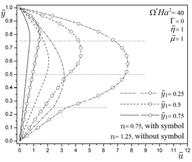
Figure 6 Dimensionless velocity profile for a purely MHD flow for different values of the interface position y¯1 and flow behavior index n. 

On the other hand, we should remember that the the fictitious interface position y¯2 represents an important aspect in flow field analysis for the power-law conducting fluid since it allows us to know the location of the maximum or minimum in the velocity profile, as well as the location where the change in sign of the velocity gradient occurs. Therefore, Table I shows the interface position y¯2 of Fig.2 and 3, while Table II displays the corresponding interface position 𝑦 2 of Fig. 4 and 5. From Tables I and II, it is determined that all the dimensionless parameters analyzed in this work influence the position of y¯2; however, the most representative for the location of this fictitious interface is the flow behavior index.

4.2.Flow rate

In Fig. 7 , the dimensionless flow rate Q¯ of a purely MHD flow is analyzed as a function of the parameter Ω*Ha2, as well as for different positions of the liquid-liquid interface y¯1. Here, Q¯T refers to the total flow rate handled by the micropump, while Q¯1 is the flow rate of the non-conducting fluid (Newtonian fluid). The driving fluid is a shear-thinning fluid with n = 0.8 and a viscosity ratio of η¯=1.2. As can be seen, the flow rate tends to increase with the increment of the parameter Ω*Ha2, reaching a maximum value when Ω*Ha2=100 and a minimum value when Ω*Ha2=0. In the absence of magnetic effects, i.e., at the hydrodynamic limit when Ω*Ha2→0, the classical Poiseuille flow can be recovered if Γ≠0 (a case that was not included in the flow rate analysis because these effects do not correspond to the main focus, which is the transport of a non-conducting fluid by viscous drag effects from a neighboring conducting fluid induced by Lorentz forces). On the other hand, the magnitude of the total flow rate Q¯T increases when the thickness of the driving fluid increases. However, this behavior is not repeated in the case of Q¯1 since the maximum flow rate is obtained when y¯1=0.5 (which occurs when the thickness of both layers is the same). The above means that Q¯1 decreases when the liquid-liquid interface position y¯1 moves away from the microchannel center. The latter effect results because when the thickness of the Newtonian fluid layer is greater (when y¯1=0.75), the driving fluid is not able to pump large amounts of liquid, and when the thickness of the Newtonian fluid layer is less (when y¯1=0.25), the amount of pumped fluid decreases due to the reduction in cross-sectional area.

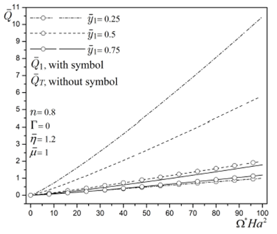
Figure 7 Dimensionless flow rate for a purely MHD flow as a function of the parameter Ω *Ha² for different values of the interface position y¯1. 

Figure 8 shows the dimensionless flow rate Q¯ of a purely MHD flow as a function of the interface position y¯1 for different values of the flow behavior index n. In the graph, the maximum total flow rates Q¯T (lines without symbols) are achieved when the thickness of the driving fluid (power-law fluid) is greater than that of the driven fluid (Newtonian fluid), which happens when y¯1→0. However, in this condition, the driven fluid (Newtonian fluid) tends to have the minimum flow rate Q¯1 (lines with symbols) because it occupies a tiny channel cross-section until reaching the condition of Q¯1=0 at y¯1=0, which corresponds to the absence of the driven fluid. In the contrary case, Q¯T and Q¯1 tend to diminish as y¯1→1 because the driving fluid is thinner, therefore diminishing the driving force to move the fluids until reaching the condition of Q¯T=0 and Q¯1=0 at y¯1=1, i.e., the absence of the driving fluid. Because the purpose of this work is to pump the non-conducting fluid (Newtonian fluid), the maximum flow Q¯1 will be obtained when the position y¯1 is located near the microchannel center, more specifically, y¯1=0.49, y¯1=0.5 and y¯1=0.52 for n = 1.25, 𝑛=1 and n = 0.75, respectively. Furthermore, it is clear that the flow rate Q¯1 increases with shear-thinning fluids.

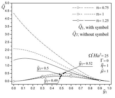
Figure 8. Dimensionless flow rate for a purely MHD flow as a function of the interface position y¯1 for different values of the flow behavior index n. 

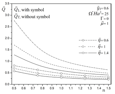
Figure 9 evaluates the dimensionless flow rate as a function of the flow behavior index, which ranges from a shear-thinning fluid of n = 0.5 to a shear-thickening fluid of n = 1.5; additionally, the analysis is performed under three flow conditions determined by the viscosity ratios of η¯=0.6,1,1.4. In this case, it is assumed that the thickness of the driving fluid layer is less than that of the driven fluid layer through a liquid-liquid interface located at y¯1=0.6 and that in the absence of a pressure gradient, the flow field is pumped only by magnetic effects given by Ω*Ha2=25. The results are prepared for both the total flow rate Q¯T and the flow rate of the driven fluid Q¯1. The graph shows that the largest flow rate values correspond to shear-thinning fluids (n < 1) up to a maximum value of n = 0.5, which then decrease when approaching the value of the shear-thickening fluid of n = 1.5.

The changes in the viscosity ratio parameter from η¯=1.4 to η¯=0.6 allow for decreased resistance of the driving fluid opposed to the flow, and consequently, higher volumetric flows are achieved. This increase is shown for Q¯T and Q¯1, indicating that in both cases, the maximum flow rate is achieved with η¯=0.6 and the minimum is achieved with η¯=1.4.

Figure 9 Dimensionless flow rate for a purely MHD flow as a function of the flow behavior index n, for different values of the viscosity ratio η¯.

References

1. U. Müller and L. Bühler, Magnetofluiddynamics in Channels and Containers (Springer, Berlin-Heidelberg, 2001), https://doi.org/10.1007/978-3-662-04405-6. [ Links ]
2. P.A. Davidson, An Introduction to Magnetohydrodynamics (Cambridge Univerity Press, New York, U.S., 2001). https://doi.org/10.1017/CBO9780511626333. [ Links ]
3. R. J. Moreau, Magnetohydrodynamics (Springer, Dordrecht, 1990), https://doi.org/10.1007/978-94-015-7883-7. [ Links ]
4. O.M. Al-Habahbeh, M. Al-Saqqa, M. Safi and T. Abo Khater, Review of magnetohydrodynamic pump applications, Alex. Eng. J. 55(2016) 1347, http://doi.org/10.1016/j.aej.2016.03.001. [ Links ]
5. V. Patel and S.K. Kassegne, Electroosmosis and thermal effects in magnetohydrodynamic (MHD) micropumps using 3D MHD equations, Sens. Actuator B-Chem. 122 (2007) 42, https://doi.org/10.1016/j.snb.2006.05.015. [ Links ]
6. I. Dolezel, V. Kotlan, B. Ulrych and V. Valenta, Magnetohydrodynamic pumps with permanent magnets for pumping molten metals or salts, Electroscope 2009 (2009) 86. [ Links ]
7. I. Dolezel, V. Kotlan and B. Ulrych, Magnetohydrodynamic pumps for molten salts in cooling loops of high-temperature nuclear reactors, Prz. Elektrotech. 2011 (2011) 28. [ Links ]
8. H. Kabbani, A. Wang, X. Luo, and S. Qian, Modeling Redoxbased magnetohydrodynamics in three-dimensional microfluidic channels, Phys. Fluids 19(2007) 083604, https://doi.org/10.1063/1.2759532. [ Links ]
9. C. Kleinstreuer, Microfluidics and Nanofluidics. Theory and Selected Applications (Wiley, New Jersey, 2013), https://doi.org/10.1002/9781118749890. [ Links ]
10. D. Li, Encyclopedia of Microfluidics and Nanofluidics (Springer, Boston, 2008). https://doi.org/10.1007/978-0-387-48998-8. [ Links ]
11. A. Homsy et al., A high current density DC magnetohydrodynamic (MHD) micropump, Lab Chip 5 (2005) 466, https://doi.org/10.1039/B417892K. [ Links ]
12. H. S. Kabbani, M. J. Mack, S. W. Joo and S. Qian, Analytical prediction of flow field in magnetohydrodynamic-based microfluidic devices, J. Fluids Eng.-Trans. ASME 130 (2008) 091204, https://doi.org/10.1115/1.2953302. [ Links ]
13. F. E. H. Tay, Microfluidics and BioMEMS Applications (Springer, Boston, 2002). https://doi.org/10.1007/978-1-4757-3534-5. [ Links ]
14. S. Lim and B. Choi, A study on the MHD (magnetohydrodynamic) micropump with side-walled electrodes, J. Mech. Sci. Technol. 23(2009) 739, https://doi.org/10.1007/s12206-008-1107-0. [ Links ]
15. L. Huang, W. Wang, M.C. Murphy, K. Lian and Z.-G. Ling, LIGA fabrication and test of a DC type magnetohydrodynamic (MHD) micropump, Microsyst. Technol. 6 (2000) 235, https://doi.org/10.1007/s005420000068. [ Links ]
16. D. Chatterjee and S. Amiroudine, Lattice Boltzmann simulation of thermofluidic transport phenomena in a DC magnetohydrodynamic (MHD) micropump, Biomed. Microdevices 13 (2011) 147, https://doi.org/10.1007/s10544-010-9480-8. [ Links ]
17. H. H. Bau, J. Zhu, S. Qian and Y. Xiang, A magnetohydrodynamically controlled fluidic network, Sens. Actuator B Chem. 88(2003) 205, https://doi.org/10.1016/S0925-4005(02)00325-8. [ Links ]
18. M. Rivero and S. Cuevas, Analysis of the slip condition in magnetohydrodynamic (MHD) micropumps, Sens. Actuator B Chem. 166-167 (2012) 884, https://doi.org/10.1016/j.snb.2012.02.050. [ Links ]
19. J. Azimi-Boulali, M. Zakeri and M. Shoaran, A study on the 3D fluid flow of MHD micropump, J. Braz. Soc. Mech. Sci. Eng. 41(2019) 478, https://doi.org/10.1007/s40430-019-1979-1. [ Links ]
20. S. Moghaddam, Investigating flow in MHD micropumps, SN Appl. Sci. 1(2019) 1609, https://doi.org/10.1007/s42452-019-1644-4. [ Links ]
21. Y. Jian and L. Chang, Electromagnetohydrodynamic (EMHD) micropumps under a spatially non-uniform magnetic field, AIP Adv. 5 (2015) 057121, https://doi.org/10.1063/1.4921085. [ Links ]
22. P. K. Mondal and S. Wongwises, Magneto-hydrodynamic (MHD) micropump of nanofluids in a rotating microchannel under electrical double-layer effect, Proc. Inst. Mech. Eng. E 234(2020) 318, https://doi.org/10.1177/0954408920921697. [ Links ]
23. S. Moghaddam, MHD micropumping of power-law fluids: A numerical solution, Korea Aust. Rheol. J. 25(2013) 29, https://doi.org/10.1007/s13367-013-0004-y. [ Links ]
24. M. Pourjafar, F. Malmir, S. Bazargan and K. Sadeghy, Magnetohydrodynamic flow of Bingham fluids in a plane channel: A theoretical study, J. Non-Newton. Fluid Mech. 264 (2019) 1, https://doi.org/10.1016/j.jnnfm.2018.12.005. [ Links ]
25. Y. A. Elmaboud and S. I. Abdelsalam, DC/AC magnetohydrodynamic-micropump of a generalized Burger’s fluid in an annulus, Phys. Scr. 94(2019) 115209, https://doi.org/10.1088/1402-4896/ab206d. [ Links ]
26. A. Shahidian et al., Flow analysis of non-Newtonian blood in a magnetohydrodynamic pump, IEEE Trans. Magn. 45(2009) 2667, https://doi.org/10.1109/TMAG.2009.2018954. [ Links ]
27. F.-Q. Li, Y.-J. Jian, Z.-Y. Xie, and L. Wang, Electromagnetohydrodynamic flow of Powell-Eyring fluids in a narrow confinement, J. Mech. 33(2017) 225, https://doi.org/10.1017/jmech.2016.75. [ Links ]
28. R. Shail, On laminar two-phase flows in magnetohydrodynamics, Int. J. Eng. Sci. 11(1973) 1103, https://doi.org/10.1016/0020-7225(73)90111-0. [ Links ]
29. J. Lohrasbi and V. Sahai, Magnetohydrodynamic heat transfer in two-phase flow between parallel plates, Appl. Sci. Res. 45(1988) 53, https://doi.org/10.1007/BF00384182. [ Links ]
30. J. C. Umavathi, A. Mateen, A.J. Chamka and A. Al-Mudhaf, Oscillatory Hartmann two-fluid flow and heat transfer in a horizontal channel, Int. J. Appl. Mech. Eng. 11 (2006) 155. [ Links ]
31. A. Mateen, Magnetohydrodynamic flow and heat transfer of two immiscible fluids through a horizontal channel, Int. J. Curr. Eng. Technol. 3 (2013) 1952. [ Links ]
32. Z. Abbas and J. Hasnain, Two-phase magnetoconvection flow of magnetite (Fe3O4) nanoparticles in a horizontal composite porous annulus, Res. Phys. 7 (2017) 574, https://doi.org/10.1016/j.rinp.2016.12.022. [ Links ]
33. Z. Abbas, J. Hasnain and M. Sajid, Hydromagnetic mixed convective two-phase flow of couple stress and viscous fluids in an inclined channel, Z. Naturforsch. A 69 (2014) 553, https://doi.org/10.5560/zna.2014-0048. [ Links ]
34. M. S. Malashetty and J. C. Umavathi, Two-phase magnetohydrodynamic flow and heat transfer in an inclined channel, Int. J. Multiph. Flow 23 (1997) 545, https://doi.org/10.1016/S0301-9322(96)00068-7. [ Links ]
35. M. S. Malashetty, J. C. Umavathi, and J. P. Kumar, Magnetoconvection of two-immiscible fluids in vertical enclosure, Heat Mass Transf. 42 (2006) 977, https://doi.org/10.1007/s00231-005-0062-x. [ Links ]
36. D. Nikodijevic, D. Milenkovic and Z. Stamenkovic, MHD Couette two-fluid flow and heat transfer in presence of uniform inclined magnetic field, Heat Mass Transf. 47 (2011) 1525, https://doi.org/10.1007/s00231-011-0815-7. [ Links ]
37. P. Chanturani and S.S. Bharatiya, Two layered magnetohydrodynamic flow through parallel plates with applications, Indian J. Pure Appl. Math. 32 (2001) 55. [ Links ]
38. A. Brask, G. Goranovi´c, M.J. Jensen and H. Bruus, A novel electro-osmotic pump design for nonconducting liquids: theoretical analysis of flow rate-pressure characteristics and stability, J. Micromech. Microeng. 15 (2005) 883, https://doi.org/10.1088/0960-1317/15/4/029. [ Links ]
39. Y. Gao, T. N. Wong, C. Yang and K. T. Ooi, Transient twoliquid electroosmotic flow with electric charges at the interface, ColloidS Surf. A. 266(2005) 117, https://doi.org/10.1016/j.colsurfa.2005.05.068. [ Links ]
40. G. D. Ngoma and F. Erchiqui, Pressure gradient and electroosmotic effects on two immiscible fluids in a microchannel between two parallel plates, J. Micromech. Microeng. 16 (2006) 83, https://doi.org/10.1088/0960-1317/16/1/012. [ Links ]
41. M. Liu and J. Yang, Electrokinetic effect of the endothelial glycocalyx layer on two-phase blood flow in small blood vessels, Microvas. Res. 78 (2009) 14, https://doi.org/10.1016/j.mvr.2009.04.002. [ Links ]
42. A. M. Afonso, M. A. Alves and F. T. Pinho, Analytical solution of two-fluid electro-osmotic flows of viscoelastic fluids, J. Colloid Interface Sci. 395 (2013) 277, https://doi.org/10.1016/j.jcis.2012.12.013. [ Links ]
43. Y. Huang, H. Li and T.N. Wong, Two immiscible layers of electro-osmotic driven flow with a layer of conducting non-Newtonian fluid, Int. J. Heat Mass Transf. 74 (2014) 368, https://doi.org/10.1016/j.ijheatmasstransfer.2014.02.068. [ Links ]
44. K. M. Joshep, A. Peter, P. E. Asie and S. Usman, The unsteady MHD free convective two immiscible fluid flows in a horizontal channel with heat and mass transfer, Int. J. Math. Comput. Res. 3 (2015) 954. [ Links ]
45. D. Nikodijevič, Ž. Stamenkovič, D. Milenkovič, B. Blagojevič and J. Nikodijevič, Flow and heat transfer of two immiscible fluids the presence of uniform inclined magnetic field, Math. Probl. Eng. 2011 (2011) 132302, https://doi.org/10.1155/2011/132302. [ Links ]
46. A. Z. Szeri, Fluid Film Lubrication 2nded. (Cambridge University Press, Cambridge, 2010), https://doi.org/10.1017/CBO9780511782022. [ Links ]
47. G. W. Sutton and A. Sherman, Engeneering Magnetohydrodynamics (Dover Publications, New York, 2006). [ Links ]
48. A. Ramos, Electrohydrodynamic and magnetohydrodynamic micro- pumps, in: S. Hardt, F. Schönfeld (Eds.), Microfluidic Technologies for Miniaturized Analysis Systems (Springer, Boston, 2007). https://doi.org/10.1007/978-0-387-68424-62. [ Links ]
49. H. Kim, H. Hwang, S. Baekand D. Kim, Design, fabrication and performance evaluation of a printed-circuit-board microfluidic electrolytic pump for lab-on-a-chip devices, A. Phys. 277 (2018) 73, https://doi.org/10.1016/j.sna.2018.04.042. [ Links ]
50. A. Homsy, Ph.D. thesis, University of Neuchâtel, 2006. 51. H.-L. Zhang and S. J. Han, Viscosity and density of water + sodium chloride + potassium chloride solutions at 298.15 K, J. Chem. Eng. Data 41(1996) 516, https://doi.org/10.1021/je9501402. [ Links ]
52. T. Isono, Density, viscosity, and electrolytic conductivity of concentrated aqueous electrolyte solutions at several temperatures. Alkaline-earth chlorides, lanthanum chloride, sodium chloride, sodium nitrate, sodium bromide, potassium nitrate, potassium bromide, and cadmium nitrate, J. Chem. Eng. Data 29 (1984) 45, https://doi.org/10.1021/je00035a016. [ Links ]
53. J. Kestin, H. Ezzat Khalifa and R. J. Correia, Tables of the dynamic and kinematic viscosity of aqueous KCI solutions in the temperature range 25-150 ±C and the pressure range 0.1-35 MPa, J. Phys. Chem. Ref. Data 10(1981) 57, https: //doi.org/10.1063/1.555640. [ Links ]
54. Y. C. Wu, W. F. Koch and K. W. Pratt, Proposed new electrolytic conductivity primary standars for KCl solutions, J. Res. Natl. Inst. Stand. Technol. 96 (1991) 191, https://doi.org/10.6028/jres.096.008. [ Links ]
55. H. Golnabi, M.R. Matloob, M. Bahar and M. Sharifian, Investigation of electrical conductivity of different water liquids and electrolyte solutions, Iran. Phys. J. 3 (2009) 24, https://www.sid.ir/en/journal/ViewPaper.aspx?id=191551. [ Links ]
56. S. Qian and H. H. Bau, Magneto-hydrodynamics based microfluidics, Mech. Res. Commun. 36 (2009) 10, https://doi.org/10.1016/j.mechrescom.2008.06.013. [ Links ]
57. F. A. Morrison, Undestanding Rheology (Oxford University Press, Oxford, 2001). [ Links ]
58. R. W. Flumerfelt, W. M. Pierick, S. L. Cooper and R. B. Bird, Generalized plane Couette flow of a non-Newtonian fluid, Ind. Eng. Chem. Fundamen. 8 (1969) 354, https://doi.org/10.1021/i160030a028. [ Links ]
59. J.D. Hoffman, Numerical Methods for Engineers and Scientists (Marcel Dekker, New York 2001). [ Links ]
60. J. Jang and S. S. Lee, Theoretical and experimental study of MHD (magnetohydrodynamic) micropump, Sens. Actuator A-Phys. 80 (2000) 84, https://doi.org/10.1016/S0924-4247(99)00302-7. [ Links ]
61. Z. P. Aguilar, P. Arumugam and I. Fritsch, Study of magnetohydrodynamic driven flow through LTCC channel with self-contained electrodes, J. Electroanal. Chem. 591(2006) 201, https://doi.org/10.1016/j.jelechem.2006.04.019. [ Links ]
Received: January 05, 2021; Accepted: June 09, 2021
Creative Commons License This is an open-access article distributed under the terms of the Creative Commons Attribution License