


 nueva página del texto (beta)
 Inglés (pdf)
 Artículo en XML
 Referencias del artículo
 Enviar artículo por email
 Citado por SciELO
  Similares en
SciELO
Similares en
SciELO 
 Permalink
1. Introduction
Valley of Mexico lies in the central part of Trans-Mexican Volcanic Belt (TMVB) which is an E-W oriented, Miocene to Quaternary, calc-alkaline volcanic arc related to the subduction of Rivera and Cocos plates below Mexico. It is traversed by faults which are parallel as well as orthogonal to its axis (Pasquaré et al., 1987; Johnson and Harrison, 1990) (Figure 1). The stress regime of the TMVB is transtensional (Mooser, 1972; Suter et al., 1992; Ego and Ansan, 2002).
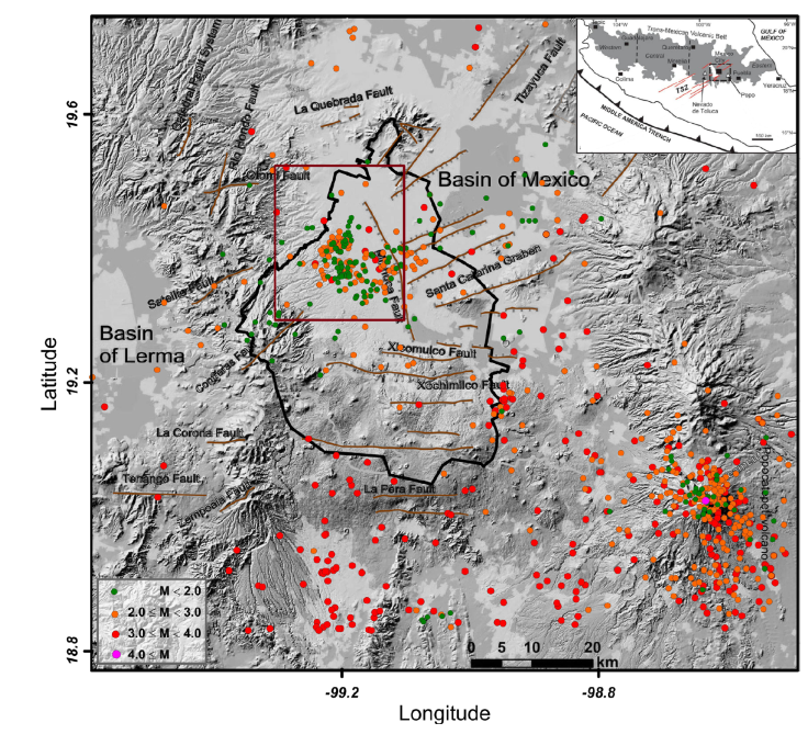
Figure 1 Digital elevation model of the Mexico Basin area showing faults in the region (modified from Arce et al., 2019). Inset: Map of central Mexico in which the thick dashed rectangle indicates the area covered by the figure. Heart-shaped black contour is Mexico City. Seismicity in the region for 2010 - May 2023 is shown by color-coded dots. Note the concentration of earthquakes within a rectangular area in the west of the city, in Milpa Alta to the south-east, and in the area of currently-active Popocatepetl Volcano. An enlarged map of the rectangular area is shown in Figure 2.
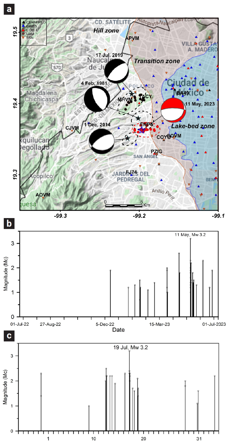
Figure 2 a) Enlarged view of the rectangular area marked in Figure 1. Hill, lake-bed, and transition zones are delineated in the figure. Dashed contours enclose seismic activity during the seismic sequence of 1981, 2014, 2019, and 2023. Star: mainshock location. Beach ball: focal mechanism. For the 2023 event the locations of the aftershocks are shown. Although recordings from 74 stations (19 in the hill zone, 14 in the transition zone, and 41 in the lake-bed zone) are analyzed in this study, only stations that are mentioned in the text are identified in the figure. b) Coda-wave magnitude versus time of events within a radius of 5 km from the epicenter of the earthquake of 11 May 2023, during a period of one year, from 1 July 2022 to 30 June 2023. Total number events = 45. Note the absence of activity during the first half of the period. c) Coda-wave magnitude versus time of events during the 2019 sequence. Much of the activity was concentrated between 12 -19 July 2019.
The valley is surrounded by volcanic ranges of andesitic and dacitic composition (Figure 1). Numerous normal faults trending E-W and NE-SW have been mapped in the region. Although the Valley of Mexico and Mexico Basin may refer to distinct areas, here we shall use the terms interchangeably; Mexico City is situated within the valley (Figure 1). Based on geotechnical characteristics of the near-surface layers, the city is divided in three zones: (1) the hill zone with surface layer of volcanic tuffs or lava flows, (2) the lake-bed zone consisting of 10 to >100 m of clays underlain by sandy and silty layers, and (3) the transition zone composed of alluvial sandy and silty layers, with occasional clay layers (Marsal and Mazari, 1969). Seismic waves suffer dramatic amplification in the lake-bed and transition zones with respect to hill zone at the natural frequency of the site, which lies between 0.2 and 0.7 Hz (Singh et al., 1988a, 1988b; Reinoso and Ordaz, 1999).
Local earthquakes in the Valley of Mexico, though small in magnitude, cause great panic in the population living in the epicentral zone. Seismicity often occurs in swarm-like sequences (Figueroa, 1971; Manzanilla, 1986). As can be seen in Figure 1, the recent events are concentrated in a rectangular area to the west, as well as at Milpa Alta to the southeast, and the area of currently-active Popocatepetl Volcano. Because of scarcity of seismic instrumentation in the Valley of Mexico, until recently only a few local earthquakes could be studied in detail. Among the well-studied events is a swarm-like activity that occurred near the seismological station of Tacubaya (TAC) in 1981 (Figure 2a) (Havskov, 1982). The swarm lasted from 4 to 15 February 1981; the largest event, M L3.3, occurred on 4 February. This figure also shows other events well recorded in this area.
The disaster suffered by Mexico City during the great Michoacán earthquake of 1985 (M w8.0) and, more recently, from the Puebla-Oaxaca inslab earthquake of 2017 (M w7.0), along with the frequently- occurring local events, have produced a rapid increase in the number of seismographs and accelerographs in the valley, installed and maintained by different institutions (Quintanar et al., 2018). For this reason, the swarm-like activity that occurred in the city in June-August 2019 was extensively recorded. This sequence also occurred close to TAC, about 4 km north of the 1981 sequence (Figure 2a). The largest event of the 2019 sequence, an M w3.2 earthquake on 17 July (Figure 2c), caused great panic in some of the neighborhoods of the city, and produced peak ground acceleration (PGA) exceeding 0.3 g at the closest station about 1 km away. Analysis of the large dataset produced by the sequence presented unusual difficulties (Singh et al., 2020) owing to the complex upper crust and highly-variable superficial layers of the Valley of Mexico.
On 11 May 2023 a local earthquake in the city was felt very strongly in Mixcoac, San Angel, and Coyoacán neighborhoods. The earthquake was preceded and followed by events that were also alarming to the population (Figure 2b). The events in the 2023 sequence were located about 5 km south of the 2019 sequence, most events occurring within 2 km of the 1981 sequence (Figure 2a). The 11 May 2023 earthquake produced a PGA triplet of (152, 139, 178 cm/s2) on the NS, EW, and Z components.
This paper presents an analysis of the 2023 sequence. We focus on the source characteristics of the main event and the recorded ground motions in the three geotechnical zones in which the city is divided. The study closely follows that of the 2019 sequence and draws on several of the results derived therein. Although there is no evidence of the magnitude of a local earthquake exceeding 4.2 since 1910, larger events can´t be ruled out as there are several mapped normal faults in the valley which exceed 20 km in length (Figure 1). Also, the TMVB has experienced many significant earthquakes in the last 450 years (Suárez et al., 2019). This emphasizes the need of careful analyses of small earthquakes in Mexico City as it may help us understand what might happen during postulated, larger earthquakes.
2. Crustal Model, Location of Events, and Moment Tensor Inversion of the Main Event
In locating the events, we only used phase data from stations at epicentral distance (Δ) ≤ 20 km. Including farther stations increases the residuals at closer stations, no doubt due to the complex and heterogeneous shallow crustal structure. (S-P) time at the nearest station ENP8 for the main event is 0.44 s, suggesting that it was a shallow earthquake, similar to those that occurred during the nearby sequences of 1981 and 2019.
The crustal model used in locating the events and in moment tensor (MT) inversion is the same as given in Singh et al. (2020) which is reproduced in Table 1. The model was developed from those reported by Havskov (1982), Cruz-Atienza et al. (2010), and Espíndola et al. (2017). P-wave velocity, α, of top two layers was taken from a refraction study (Havskov and Singh, 1978). For the near-source data analyzed here, the waves mostly traverse through the first two layers. From P and S arrival times from the 2019 earthquake sequence and construction of the Wadati diagram, Singh et al. (2020) estimated α /β = 1.84, hence β in the first layer of 1.58 km/s. The low β of the first layer may be consequence of high-water content of the rocks. For other layers α/β was fixed at 1.73. Density (ρ) and S -and P-wave quality factors (Q β and Q α ), listed in the Table 1, have been chosen in agreement with values reported by Havskov (1982) for that zone of the city; MT inversion is not sensitive to an accurated value of these parameters.
Table 1 Crustal Model (from Singh et al., 2020)
| Layer | Thickness, km | α, km/s | β, km/s | ρ, gm/ cm3 | Qβ1 |
|---|---|---|---|---|---|
| 1 | 2 | 2.90 | 1.58 | 2.50 | 50 |
| 2 | 2 | 4.70 | 2.72 | 2.76 | 50 |
| 3 | 26 | 6.60 | 3.81 | 2.82 | 50 |
| 4 | 5 | 7.10 | 4.10 | 3.03 | 50 |
| 5 | ∞ | 8.10 | 4.68 | 3.14 | 150 |
1Qα=2Qβ
Seismograms of some selected events of the sequence at the closest station ENP8 are displayed in Figure 3. Clearly, the recording of the main event is contaminated by a smaller earthquake which occurred 2.7 s earlier (top trace). This made reading of the first motions difficult. The contamination also affects the MT inversion of the main event as the signal includes contribution from both events. A few other events were also preceded by a smaller event (Figure 3).
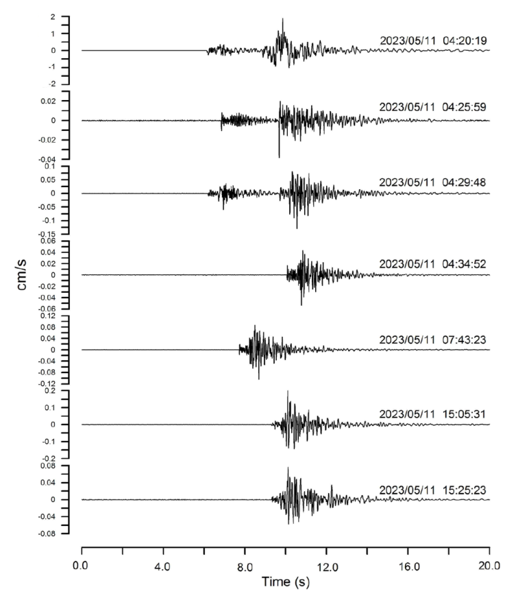
Figure 3 Velocity seismograms (cm/s) of the mainshock and some of the aftershocks at the closest station ENP8 (Z component). The mainshock (top trace) was preceded by a relatively small event that occurred 2.7 s earlier. A few other events were also preceded by a small event (second and third traces from the top).
The events were located using SEISAN program (Havskov and Ottemöller, 1999). The hypocentral parameters of the main event are: 19.364°N, 99.197°W, H = 0.8 km, origin time 04:20:19.4, residual 0.37 s. Although the aftershock activity was intense, only 30 of these events were large enough to be located; the hypocenters of 22 of these could be determined using the double-difference technique (Waldhauser and Ellsworth, 2000). The locations are shown in Figure 2a.
Moment tensor inversion for the mainshock was performed using algorithm ISOLA (Sokos and Zahradnik, 2008). The algorithm allows for the inversion of complete regional and local waveforms. The moment tensor is retrieved through a least-squares inversion, whereas the position and origin time of the point sources are grid searched with a correlation coefficient greater than 90%. Green’s functions, which includes near-field contribution, are calculated using the discrete wavenumber method (Bouchon, 1981; Coutant, 1989).
ISOLA has different error parameters that quantify the uncertainty of each solution. Each one of these parameters is not significant on its own; a joint interpretation of all the parameters is recommended (Sokos and Zahradnik, 2013). A useful indicator of solution quality is the Focal-Mechanism Variability Index, (FMVAR), defined as the mean K- angle (Kagan, 1991) of all acceptable solutions (as specified by the user-defined correlation threshold) with respect to the best-fit solution. A large value of FMVAR indicates that the moment tensor is unstable; conversely, when the focal mechanism is stable in the neighborhood of a source with maximum correlation, FMVAR will have a small value (Sokos and Zahradnik, 2013).
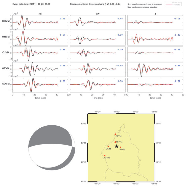
After many trials with different sets of stations, we used band-passed (0.08 - 0.24 Hz) displacement seismograms at stations COVM, MHVM, CJVM, APVM, and AOVM (Figure 4) in the inversion. The epicenter was fixed at the location obtained from the phase data. The Green’s functions were generated using the crustal model given in Table 1. Observed and synthetic wave-forms are shown in the figure. The retrieved source parameters are: M0 = 6.79 × 10¹³ Nm (M w3.2), H = 0.7 km, and NP1: φ = 270°, δ = 76°, λ = −75°; NP2: φ = 42°, δ = 20°, λ = −136°. The quality of the solution is moderate as seen from the fit of the synthetic seismograms to observed ones and by the FMVAR value of 22±21. The moderate quality of the solution is partly due to the contamination of the signal by an event that preceded the main event and partly due to the inadequacy of the 1-D crustal model to represent the real complex 3-D crustal structure. Based on the orientation of the faults mapped in the valley (Figure 1) and focal mechanisms of other events in the vicinity (Figure 2a), our preferred fault plane is NP1.
3. Source Spectrum, Variability of Ground Motion, and Site Effect
A theoretical source spectrum of the 11 May 2023 earthquake may be constructed from the seismic moment, M 0, estimated from the MT inversion, and an estimate of the stress drop, Δσ. To predict ground motion from future earthquakes it is important to know if the source spectrum computed from the observed recordings agree with the theoretical source spectrum. We first briefly present the procedure we have used to compute the source spectrum from the observed data.
The Fourier acceleration spectrum, A(f, R), of horizontal component of S-wave group at a site in the far-field may be written as:
where Ṁ
0(f) is the source displacement spectrum (also called the moment rate spectrum) so that Ṁ
0(f) → M
0 as f → 0, R = hypocentral distance, R
θcφ
= average radiation pattern (0.55), F = free surface amplification (2.0), P takes into account the partitioning of energy in the two horizontal components (
where f c is the corner frequency. In Brune source model the stress drop, Δσ, is related to M 0 and f c by (Brune, 1970):
4. Corner Frequency and Stress Drop
It is difficult to estimate the corner frequency fc (hence, Δσ from Equation 2b) from the source spectrum because of the distortion caused by site effect. Yet, a knowledge of Δσ is critical to gauge the strength of the relatively shallow faults (H ~ 1 km) in the Valley of Mexico. It is also a crucial parameter in the estimation of ground motion from postulated earthquakes.
An alternative method to estimate f c is from the ratio of spectrum of a small event to that of the mainshock. The small event and mainshock should be collocated and should have the same focal mechanism. We could find only one suitable small event, an earthquake that occurred on 21 April 2023 (M c2.6). It was well recorded at stations PZIG, COVM, and COYO (Figure 2a). Figures 5a,b,c show the ratios of the NS, EW, and Z components as well as the geometric mean of the ratios of the three components at each of these stations. All nine spectral ratios and their geometric mean curve are displayed in Figure 5d. Each frame includes the theoretical spectral ratio corresponding to an ω -2, constant Δσ, source model, a moment ratio of 10-2, and corner frequencies, f c, of 1.44 Hz (Δσ = 0.5 MPa) and 0.84 Hz (Δσ = 0.1 MPa). Short vertical lines in the figure mark f c of 1.44 and 0.84 Hz. The observed ratios point to f c = 1.44 Hz (Δσ = 0.5 MPa) for the mainshock albeit with considerable uncertainty.
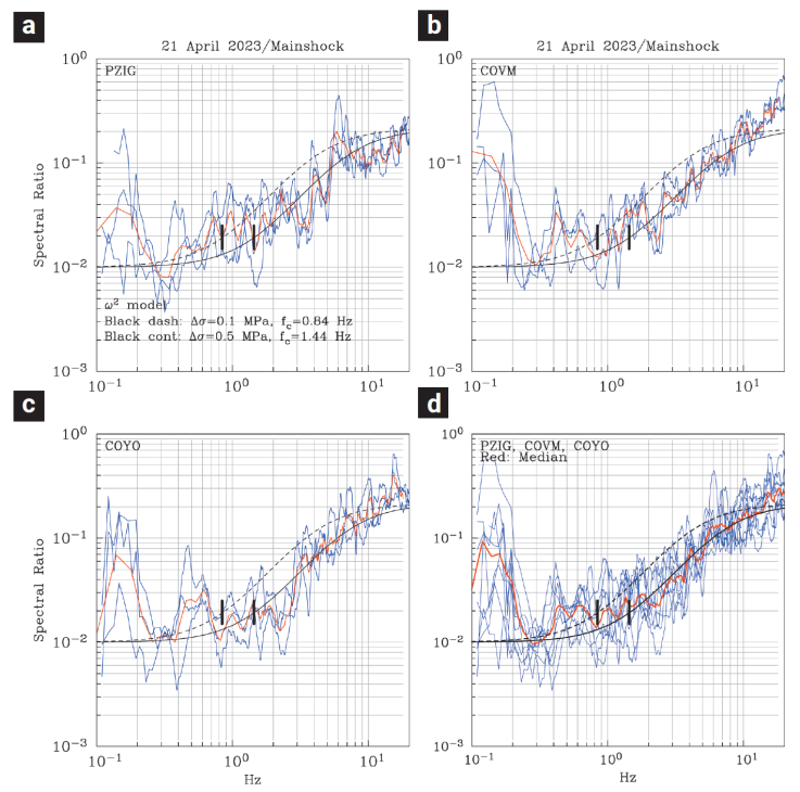
Figure 5 Spectral ratios of the earthquake of 21 April 2023 to the mainshock of 11 May 2023 at a) PZIG, b) COVM, c) COYO. Red curve is the geometric mean of NS, EW, and Z ratios. d) Geometric mean curve (in red) of spectral ratios at PZIG, COVM, and COYO. Each frame shows theoretical spectral ratio corresponding to an ω -2, constant Δσ source model, a moment ratio of 10-2, and corner frequency, f c, of 1.44 Hz (Δσ = 0.5 MPa) (black smooth curve) and 0.84 Hz (Δσ = 0.1 MPa) (black, dashed, smooth curve). Short vertical lines mark f c of 1.44 and 0.84 Hz. Observed ratios suggest fc = 1.44 Hz (Δσ = 0.5 MPa) for the mainshock.
5. Source Spectrum and Site Effect
We correct the Fourier acceleration spectrum, A(f, R), at each station according to Equation 1 and solve for [f 2 Ṁ 0(f) Site(f)] which we call the observed acceleration source spectrum, OASS(f). Since M 0 and f c are known, the theoretical source spectrum, [f 2 Ṁ 0(f)], is constructed assuming a Brune ω -2 source model (Equation 2a). OASS(f) curves of the main-shock computed at 19 stations in the hill zone, 14 stations in the transition zone, and 41 stations in the lake-bed zone are illustrated in Figures 6a,b,c, respectively. The plots show remarkable variability of ground motion in each of the three geotechnical zones. Figures 6a,b,c include the geometric mean and ± one standard deviation curves. Figure 6d illustrates geometric mean curves for the sites in the hill, transition, and lake-bed zones. The figure also shows the curve at CU which is often used as a reference site. Theoretical curve for an ω -2-Brune source with Δσ of 0.5 MPa is plotted in Figures 6a,b,c,d. Ratios of the OASS(f) geometric mean curve for each zone to the theoretical [f 2 Ṁ 0 (f)] (Equation 2a) are illustrated in Figure 6e. The ratio gives Site(f), which includes amplification of the seismic waves caused by low-velocity layers above the source. For comparison, Site(f) in the hill zone, reported previously from a similar analysis of the recordings from the earthquake of 17 July 2019 earthquake (Singh et al., 2020), is also shown in Figure 6e. The difference in the two site effects is partly because the stations and their total amount were not the same in the two analyses. Note that a deviation of the source from the assumed theoretical source model and error in the estimated Δσ are mapped in the site effect.
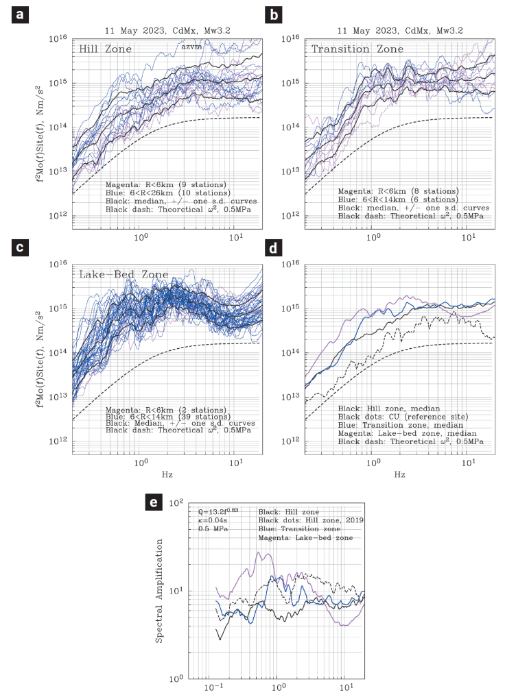
Figure 6 [f 2 Ṁ 0 (f)Site (f)] curves of the mainshock estimated at a) 19 individual stations in the hill zone, b) 14 stations in the transition zone, and c) 41 stations in the lake-bed zone. Plots show remarkable variability of ground motion in each of the three geotechnical zones. Geometric mean and ± one standard deviation curves are shown in black. d) Geometric mean curves for the sites in the hill, transition, and lake-bed zones. Also shown is the curve at CU which is often used as a reference site (dotted black line). Theoretical curve for an ω -2-Brune source with Δσ of 0.5 MPa is shown in a) to d). e) Ratios of the observed [f 2 Ṁ 0 (f)] geometric mean curve for each zone to the theoretical [f 2 Ṁ 0 (f)] curve predicted by the ω -2-Brune source model. The ratio yields Site(f), the site effect. For comparison, the site effect in the hill zone reported previously from a similar analysis of the recordings from the earthquake of 17 July 2019 earthquake (Singh et al., 2020) is also shown.
Large site effect even in the hill zone of the Valley of Mexico is not unexpected. It was previously reported by Ordaz and Singh (1992) and Singh et al. (1995) based on seismograms from coastal earthquakes recorded in the valley.
6. Observed and Predicted PGA and PGV
As discussed above, the estimation of the generic site effect in the different geotechnical zones of the Valley of Mexico depends on Δσ. However, in the present case, the estimation of ground motion from postulated events via stochastic method (Boore, 1983) does not require a knowledge of true Δσ provided that the postulated earthquake also follows the ω -2 source model, and Δσ is the same as that of the M w3.2 event. In this case, the predicted Fourier amplitude spectrum at a generic site from the postulated earthquake and, hence, also the predicted ground motion parameters remain the same irrespective of Δσ. We take advantage of this possibility and compute PGA and PGV for M w3.2 and 5.0 earthquakes. Predictions for an M w3.2 earthquake permit comparison with the observed data, while those for an M w5.0 event provide an estimate of ground motions from a reasonable scenario earthquake.
We recapitulate the assumptions made and parameters used in the application of the stochastic method: Brune ω -2 source; Δσ = 0.5 MPa; β = 1.58 km/s; ρ = 2.50 gm/cm3; κ = 0.04 s; Rx = 3 km; Q(f)=13.2f 0.83. Generic Site(f) for the three zones are shown in Figure 6e. Application of the stochastic method also requires an estimation of the effective duration, T d, of the ground motion; we use the relation (T d -1/ f c) = 0.93 Δ, where Δ is the epicentral distance; this relation was derived for the hill zone in the previous study of the 2019 sequence (Singh et al., 2020); we assume that this relation holds for all three zones. Figures 7a,b show predicted PGA and PGV curves as a function of R for an M w3.2 earthquake superimposed on the observed values. Predicted PGA curves for the three zones are nearly the same. The observed PGA values in the hill zone are in good agreement with the prediction but not in the transition and lake-bed zones where they are somewhat greater than the predicted ones. Unlike predicted PGA curves, the PGV curves for the three zones differ substantially. Both the observations and the predictions are greater for the lake-bed zone than for the transition zone which, in turn, are greater than for the hill zone. There is large scatter in the observed PGA and PGV data which is consistent with great variability of the source spectrum seen in Figures 6a,b,c.
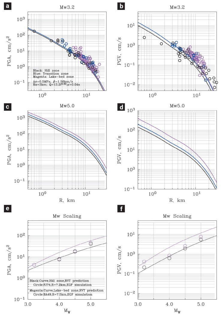
Figure 7 a), b) Predicted PGA and PGV curves for an M w 3.2 earthquake for the three geotechnical zones computed via the stochastic method superimposed on the observed values during the 2023 mainshock. c), d) Predicted PGA and PGV curves for a postulated M w 5.0 earthquake applying the stochastic technique. e), f) Predicted PGA and PGV curves as function of M w at R = 7.5 km at a generic site in the hill-zone zone and lake-bed zone using the stochastic method. Superimposed are estimated values at FJ74 (in the hill zone) and BA49 (in the lake-bed zone) using an EGF technique. Stations are located at nearly the same distance (R = 7.5 km). EGFs are the 2023 mainshock recordings at these two stations.
7. Ground Motion from a Scenario Mw5.0 Earthquake
We consider a scenario local earthquake of M w5.0 although larger earthquakes are certainly plausible because there are several mapped normal faults in the Valley of Mexico exceeding 20 km in length (Figure 1). There is, however, no evidence of an M > 4.2 local earthquake in Mexico City in the available seismograms recorded in the city (at Tacubaya for the period 1910 - 1973; at other stations since then). We estimate ground motions from the scenario earthquake by applying the stochastic technique. The technique assumes that the far-field, point source approximation is valid, i.e., distance to station, R, is much greater than both the source dimension as well the wavelength of interest. Expected rupture length of an M w5.0 earthquake is about 3 to 4 km (Wells and Coppersmith, 1994). The period of interest in Mexico City is less than about 2.5 s, so that, for β = 1.58 km/s, the wavelength of interest is < 4.0 km. It follows that for far-field approximation to be valid R should be much greater than 4.0 km. Although we present expected ground motions at shorter distances, the results for R < 6.0 km are likely to be approximate. Furthermore, the rupture of an M w5.0 earthquake may reach 3 to 4 km in depth while the parameters we have used in the simulations were estimated from shallower sources. With these limitations in mind, the expected PGA and PGV at the epicenter of a postulated M w5 earthquake are 0.6 g and 60 cm/s at a typical hill site; at lake-bed site the expected values are twice as large (Figures 7c,d). We note that the simulated PGA values at soft sites for an M w 5.0 earthquake are greater than at hard sites by a factor greater than those observed during the M w 3.2 mainshock (compare Figures 7a and 7c). It is further accentuated for PGV (compare Figures 7b and 7d). This implies that the scaling of PGA and PGV with M w differs for hard and soft sites. It is confirmed from Figures 7e and 7f which show the scaling of PGA and PGV with M w at generic sites in the hill and lake-bed zones with R fixed at 7.5 km. The figures show greater dependence of PGA and PGV on M w at the soft site. We also computed expected PGA and PGV at R = 7.5 km as a function M w using the recordings at the hill-zone station of FJ74 (R = 7.2 km) and lake-zone station of BA49 (R = 7.5 km) as empirical Green´s functions (EGFs). A scheme of random summation of EGF introduced by Ordaz et al. (1995) was used in the simulation. A stress drop of 0.5 MPa was assumed for both the EGF and target events. The predicted values from the EGF technique are superimposed in Figures 7e,f. While the stochastic predictions at hill zone and lake-bed zone differ significantly, the EGF predictions are nearly the same. This is because the predictions using EGF technique are site specific (for FJ74 and BA49) while those obtained from stochastic method are for a generic site.
Numerical modelling of wave propagation in Mexico City from local earthquakes has been the topic of two recent studies (Cruz-Atienza et al., 2016; Hernandez-Aguirre et al., 2023). These studies shed light on the cause of long coda observed in the seismograms of lake-bed zone and on the nature of the wavefield. Hernandez-Aguirre et al. (2023) computed synthetic seismograms (low-pass filtered at 1.3 Hz) from the 17 July 2019 M w 3.2 earthquake. Although the complex 3D structure of the valley is still poorly known, Hernandez-Aguirre et al. (2023) find good agreement between simulated and observed velocity records. As our knowledge of the structure improves, it will become possible to synthesize ground motions from postulated, larger earthquakes.
8. High PGA in the Epicentral Area but No Damage
As mentioned earlier, the PGA triplet on the NS, EW, and Z components during the 2023 earthquake at the epicentral station of ENP8 was (152, 139, 178 cm/s2). The corresponding triplet during the 2019 earthquake at the nearest station of MHVM was (101, 314, 305 cm/s2). No wonder these earthquakes were very strongly felt in the epicentral area. Yet, surprisingly, no building damage was reported. The epicenter of the 2019 event coincides with a cemetery. Thus, it may be argued that the absence of damage was due to the lack of structures in the epicentral region. However, no structural damage was reported during the 2023 event either although the epicentral region was located within a highly-populated zone with many one- to two-stories structures that, in principle, were susceptible to the short-period ground motion. A relevant question is whether the observed SA (pseudo response spectra, 5% damping) during the two earthquakes exceeded the design spectrum for the hill zone as prescribed in the Mexico City Building Code. Figure 8 shows the comparison. Clearly, the observed SA at short periods exceeded the design spectrum, (see also Ordaz et al., 2023). Further studies are warranted to understand the cause of the lack of structural damage during the 2019 and 2023 M w 3.2 earthquakes.
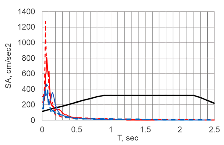
Figure 8 Comparison of recorded SAs during the 2019 and 2023 M w 3.2 earthquakes at the closest station with the design spectrum prescribed in the Mexico City Building Code for the region. The quadratic mean of the SA of the two horizontal components and the SA of the vertical component are plotted with continuous and dashed curves (blue: 2023 earthquake; red: 2019 earthquake). Continuous black line is the horizontal design spectrum according to the Mexico City Building Code.
9. Discussion and Conclusions
The earthquake of 11 May 2023 occurred in the west of Mexico City during a seismic sequence that had initiated 5 months earlier. The events in the sequence were shallow (H ~ 1 km). The earthquake was felt very strongly in Mixcoac, San Angel, and Coyoacán. The PGA at the closest station was ~ 0.18 g.
Moment tensor inversion of bandpass filtered (0.08 - 0.24 Hz) displacement records of the 2023 earthquake yields M0 = 6.8×10¹³N-m (M w 3.2), H = 0.7 km, and the likely fault plane characterized by φ = 2700, δ = 760, λ = -750.
Spectral analysis of the recordings reveals great variability of ground motion within each of the three geotechnical zones in which Mexico City is divided. The cause of this variability is clearly the complex, 3D structure of the superficial layers; hence, the parameters needed to correct the spectra of observed ground motion in Mexico City to estimate the source spectrum are not well constrained. Using those that were derived from the analysis of the earthquake of 17 July 2019, we determined the source spectrum of the 2023 event. We find a large disparity between the observed source spectrum and theoretical source spectrum (computed for an ω -2 source with Δσ = 0.5 MPa). Although we attribute this disparity to the amplification of seismic waves as they travel upwards from the source through layers of decreasing velocity, the uncertainty in the parameters used may also partly be responsible. Predicted PGA and PGV for an M w3.2 earthquake, computed using stochastic technique, assuming a Brune ω -2 source, Δσ = 0.5 MPa and including the site effect, are in reasonable agreement with the observations. Expected PGA and PGV at the epicenter of a postulated M w5 earthquake, under several assumptions, are 0.6 g and 60 cm/s at a generic hill site; at lake-bed site the expected values are twice as large.
In many respects the Mexico City earthquakes of 11 May 2023 and 17 July 2019 were very similar: (1) They occurred in the same part of the city, both were shallow (H ~ 1 km), and had the same magnitudes, M w3.2. (2) Both earthquakes were part of a swarm-like activity. (3) They were strongly felt by the population living in the epicentral area, causing panic, and producing high PGA (0.18 g in 2023; 0.3 g in 2019). (4) The response spectrum of both events at the closest station exceeded the City´s design spectrum at short periods. Even so, neither of the two events caused structural damage although there were many one- and two-story buildings in the epicentral zone (at least during the 2023 event; the epicenter of the 2019 earthquake fell in a cemetery) susceptible to ground motion at short periods. (5) As expected from transtensional stress regime of the central TMVB, both events had predominantly normal-faulting focal mechanism. (6) Stress drop of both events was low which is reasonable for these shallow events; Δσ estimate, however, is poorly constrained. A reliable estimate of Δσ of these shallow earthquakes is most desirable. (7) A large disparity between observed and theoretical source spectra is found during both earthquakes. We have attributed this to a site effect. The cause, however, could partly be the error in the parameters used in correcting the spectra.
Not all the seismicity in the Valley of Mexico is shallow. SSN earthquake catalog and examination of seismograms suggest that it extends up to a depth of ~ 15 km. These relatively deep earthquakes have yet to produce extensive recordings. Once such recordings become available it will be interesting to compare these events with the shallower ones.
10. Data and Resources
Data used in this study were obtained by the National Seismological Service (SSN; http://www.ssn.unam.mx/doi/networks/mx/), Instituto de Geofísica, UNAM; the Strong Ground Motion Database System (http://aplicaciones.iingen.unam.mx/AcelerogramasRSM/); and the Centro de Instrumentación y Registro Sísmico (CIRES; http://cires.org.mx/registro_es.php), Mexico City.

