Original papers
Love wave in porous layer under initial stress over heterogeneous elastic half-space under gravity and initial stress
Asit Kr. Gupta1
Anup Kr. Mukhopadhyay2
Pulak Patra3
*
Santimoy Kundu4
1Department of Physics, Asansol Engineering College, Asansol, India
2Department of Computer Science, Asansol Engineering College, Asansol, India
3Department of Mathematics, Brainware Group of Institutions-SDET, Kolkata, India
4Department of Applied Mathematics, IIT (ISM), Dhanbad, Jharkhand, India
Abstract
In the present paper, the effect of initial stresses and gravity on the propagation of Love waves have been studied in porous layer surface over a heterogeneous half-space. We have considered two types of boundary on free surfaces: (a) rigid boundary and (b) traction free boundary. The propagation of Love waves has been investigated under assumed media in both the cases of boundary and discusses a comparative study of two cases. The dispersion equations and phase velocities have been obtained in both cases. The numerical calculations have been done and presented graphically. This study of Love waves in the assumed medium reveals that the presence of initial stress in the half-space and absence of initial stress in the layer, the displacement of phase velocity in a rigid boundary is more than the traction free boundary.
Key words. Love wave; propagation; initial stress; heterogeneous; porous and gravity
Resumen
En este trabajo se estudió el efecto de las tensiones iniciales y la gravedad sobre la propagación de las ondas de Love, lo anterior en la superficie de una capa porosa sobre un semiespacio heterogéneo. Se consideraron dos tipos de límite en superficies libres: (a) límite rígido y (b) límite libre de tracción. La propagación de las ondas de Love ha sido investigada bajo supuestos medios, tanto en los casos de frontera como en un estudio comparativo de dos casos. En ambos, se obtuvieron las ecuaciones de dispersión y las velocidades de fase. Se presentan los cálculos numéricos de forma gráfica. Este estudio de las ondas de Love en el medio supuesto revela que la presencia de tensión inicial en el medio espacio y la ausencia de tensión inicial en la capa, el desplazamiento de la velocidad de fase en un límite rígido es mayor que el límite libre de tracción.
Palabras clave: Ondas de Love; propagación; tensión inicial; heterogéneo; poroso y gravedad
Introduction
The stress is generally developed in media due to natural phenomena. Since the earth is an elastic solid medium under high initial stresses. These stresses play a significant role to propagate an elastic wave. Chattopadhyay et al. (1978) discussed the propagation of Love type waves in an initially stressed crustal layer having an irregular interface. Chakraborty et al. (1981) shows that Love waves propagate in dissipative media under gravity. Chakraborty et al. (1983) discussed the effect of initial stress and irregularity on the propagation of SH-waves. Dey et al. (1996) discussed the propagation of Love waves in heterogeneous crust over a heterogeneous mantle. Abd-Alla et al. (1999) have studied the propagation of Love waves in a non-homogeneous orthotropic elastic layer under initial stress overlying semi-infinite medium. Dey et al. (2004) also studied the propagation of Love waves in an elastic layer with void pores. Sharma (2004) established a mathematical expression about wave propagation in a general anisotropic poroelastic medium with anisotropic permeability phase velocity and attenuation. Kalyani et al. (2008) have made finite-difference modeling of seismic wave propagation in monoclinic media.
Many researchers in the field of elastic wave propagation in layered medium bounded by different forms of irregular boundaries have been studied in several research papers. Such as Anjana and Samal (2010) shows that Love waves propagate in a fluid-saturated porous layer under a rigid boundary and lying over elastic half-space under gravity. Chattaraj and Samal (2013) investigated the propagation of Love waves in the fiber-reinforced layer over a gravitating porous half-space. Gupta et al. (2013a) discussed the propagation of Love waves in a non-homogeneous substratum over an initially stressed heterogeneous half-space. Gupta et al. (2013b) were introduced the possibility of Love wave propagation in a porous layer under the effect of linearly varying directional rigidities. SH-type waves dispersion in an isotropic medium sandwiched between an initially stressed orthotropic and heterogeneous semi-infinite media were studied by Kundu et al. (2013). Manna et al. (2013) show the Love wave propagation in a piezoelectric layer overlying in an inhomogeneous elastic half-space. Bacigalupo and Gambarotta (2014) discussed second-gradient homogenized model for wave propagation in heterogeneous periodic media. Propagation of Love wave in fiber-reinforced medium lying over an initially stressed orthotropic half-space was formulated by Kundu et al. (2014).
In this paper, we have studied the problem of propagation of Love waves in a porous layer over a heterogeneous elastic half-space under gravitating half-space for a rigid boundary as well as traction free boundary in the upper layer. Both the layer is considered under the effect of initial stress. The dispersion relations have been derived for rigid boundary as well as traction free boundary. The initial stresses play a vital role on the propagation of Love waves in the assumed medium. Gravity and heterogeneity in the half-space play a notable effect on the propagation of Love waves in the medium and half-space. The influences of porosity, initial stresses, and gravitational parameters have discussed graphically.
Formulation of the Problem
We consider a model consisting of the water-saturated anisotropic poroelastic layer under initial stress of finite thickness laying (Figure 1 under traction free boundary and Figure 2 under rigid boundary) over a gravitating heterogeneous elastic half-space under initial stress. Considering the origin of the coordinate system at the interface of the crust and mantle, z-axis downloads positively. The following variation has been taken.
For the half-space μ=μ2(1+a1z),ρ=ρ2
where, μandρ is the rigidity and density of the half space,a be the constant having inverse of length.
Solution of the Porous Layer
For the fluid-saturated anisotropic porous layer under initial stress P1 in the absence of body forces, the equation of motion can be written as (Biot, 1965).
∂s21'∂x+∂s22'∂y+∂s23'∂z-P1∂ωz∂x=∂2∂t2(ρ11vy'+ρ12Vy)∂S∂y=∂2∂t2(ρ12vy'+ρ22Vy)s23'=2Leyz,s12'=2Nexy,s22'=(A-2N)exx+Aeyy+Fezz+Qε
(1)
where, sij' are the components of stress tensor in the solid, S(=-fp) is the reduced pressure of the fluid, p is the pressure in the fluid, and f is the porosity of the porous layer, (ux',vy',wz') are the components of the displacement vector of the solid and (Ux,Vy,Wz) are those of fluid. L and N are represent the shear moduli of the anisotropic layer in the x- and z- direction respectively, whereas A and F are elastic constants for the medium. The positive quantity Q is the measure of coupling between the changes in the volume of solid and liquid.
Since the Love waves propagating along the x-direction, having the displacement of particles along the y-direction, we have
ux'=0,vy'=vx,z,t,wz'=0
Ux=0,Vy=V(x,z,t),Wz=0
This displacement will produce eyz and exy strain components and others are vanishing.
The dynamic components ρ11,,ρ12,ρ22 take into account the inertia effects of the moving fluid and are related to the densities of the solid ρs , fluid ρf and the layer ρ' by the equations
ρ11+ρ22=(1-f)ρs,ρ12+ρ22=fρf
So that the mass density of the aggregate is
ρ'=ρ11+2ρ12+ρ22=ρs+f(ρf-ρs)
Also
ρ11>0,ρ12≤0,ρ22>0,ρ11ρ22-ρ122>0
The Love wave equation takes the form
(N-P12)∂2v∂x2+L∂2v∂z2=∂2∂t2ρ11v+ρ12Vand∂2∂t2ρ12v+ρ22V=0
(2)
Hence, we have from (2)
(N-P12)∂2v∂x2+L∂2v∂z2=d1∂2v∂t2whereㅤd1=ρ11-ρ122ρ22,V=(d2-ρ12v)/ρ22,d2=[ρ12v+ρ22V]
(3)
The shear wave velocity in the porous layer along the x-direction can be expressed as
β'=N-P12d1=β11-ξ1d
whereㅤd=γ11-γ122γ22,β1=Nρ', is the velocity of shear wave in the corresponding initial stress free non-porous, anisotropic, elastic medium along x-direction.
ξ1=P12N , is the non-dimensional parameter due to the initial stress P1 and
γ11=ρ11ρ',γ12=ρ12ρ'andγ22=ρ22ρ', are the non-dimensional parameter for the material of the porous layer as obtained by Biot (1965)
We consider
v(x,z,t)=f(z)ei(kx-ωt)
(4)
where, k is the wave number and ω is the angular frequency.
Now, we get
d2f(z)dz2+q12f(z)=0,whereㅤq12=k2Lc2d-N-P12=k2αdc2β12-1-ξ1d,α=NL,ω=kc
(5)
The solution of equation (5)
f(z)=Aeiq1z+Be-iq1z
(6)
where A andB are constants
Hence, finally we get
v1(x,z,t)=(Aeiq1z+Be-iq1z)ei(kx-ωt)
(7)
The Dynamic Equation of the Motion in the Half-Space
The dynamic equation of motion in the half space may be written as Biot (1965)
∂S12∂x+∂S22∂y+∂S23∂z-ρgω23+ρgz∂ω12∂x-ρgz∂ω23∂z-P22∂v∂x2=ρ∂2v2∂t2
(8)
where, v2x,z,t is the displacement along y direction, ρ is the density, Sij are incremental stress and ωij are rotational components in the half space and g is the acceleration due to gravity. P2, is the initial stress.
The components of body forces are X=0,Y=0,Z=g.
The stress-strain relations are
S12=2μexy,S23=2μeyz,eij=12∂ui∂xj+∂uj∂xi
exy=12∂v1∂y+∂v2∂x,eyz=12∂v2∂z+∂v3∂y
In this problem ∂∂y=0 and μ=μ21+a1z,ρ=ρ2 , the stress strain relation becomes
exy=12∂v2∂x,eyz=12∂v2∂zS12=μ21+a1z∂v2∂x,S23=μ21+a1z∂v2∂z
(9)
where, μ is the modulus of rigidity, α1 is a variation parameter of a rigidity having dimension inverse of length.
Equation (8) using the above relations takes the form
μ21+a1z-12ρ2gz-P22∂2v2∂x2+μ21+a1z-12ρ2gz∂2v2∂z2+a1μ2-12ρ2g∂v2∂z=ρ2∂2v2∂t2
(10)
The solution of equation (10) may be taken as
v2=ϕzeikx-ωt
(11)
Equation (10) is now
μ21+a1z-12ρ2gz-P22-k2φ+μ21+a1z-12ρ2gzφ″+a1μ2-12ρ2gφ'+ρ2c2k2φ=0
φ″+ka1k-G21+ka1k-G2zφ'+k2c2c22-P22μ21+ka1k-G2z-1φ=
(12)
where c22=μ2ρ2,ω=kc and G=ρ2gμ2k , is the Biot’s gravity parameter, ϕ″=∂2ϕ∂z2,ϕ'=∂ϕ∂z.
Now we substitute, φz=ϕz1+ka1k-G2z12 in equation (12), we have
φ″+k2a1k-G2241+ka1k-G2z2+k2c2c22-P22μ21+ka1k-G2z-1φ=0
(13)
Using dimensionless quantities, η=-21+ka1k-G2za1k-G2
Equation (13) becomes
∂2ϕη∂η2+-14+Rη+14η2ϕη=0whereㅤR=-c2c22+P22μ22a1k-G2
(14)
which is standard Whittaker’s equation and solution is
φη=DWR,0η+EW-R,0-η
(15a)
where, DㅤandㅤE are arbitrary constants and WR,0η ,and W-R,0-η are the Whittaker functions.
As the solution should vanish at z→∞, i.e. for η→-∞, we may take the solution as
φη=W-R,0-η
(15b)
Hence
v2=EW-R,021+ka1k-G2za1k-G21+ka1k-G2z12eikx-ωt
(16)
Boundary Conditions and Dispersion Relation
We consider two cases
Case A: If the surface of the upper layer is rigid boundary, then
i.
v1=0atz=-H
ii.
Δfy1=Δfy2atz=0
iii.
v1=v2atz=0
Case B: If the surface of the upper layer is traction free, then
i.
Δfy1=0atz=-H
ii.
Δfy1=Δfy2atz=0
iii.
v1=v2atz=0
For case A using the boundary condition (i), we have
Ae-iq1H+Beiq1H=0atz=-H
(17)
For case B using the boundary condition (i), we have
Ae-iq1H-Beiq1H=0atz=-H
(18)
For case A and case B using the boundary condition (ii), we have
Liq1A-iq1B=μ2ddzEW-R,021+ka1k-G2za1k-G2eikx-ωt1+ka1k-G2z12z=0
(19)
For case A and case B using the boundary condition (iii), we have
A+B-EW-R,0-ηz=0=0
(20)
Case I -In rigid boundary, eliminating A, B and E from equation (17), (19) and (20), we have
e-iq1Heiq1H0Liq1-Liq1-μ2ddzW-R,021+kak-G2za1k-G2eikx-ωt1+ka1k-G2z12z=011-W-R,0-ηz=0=0
(21)
Expanding the determinant, we get
tanαdc2β12-1-ξ1dkH= Lμ2αdc2β12-1-ξ1d1-18-c2c22+ξ2a1k-G2+12a1k-G21-18-c2c22+ξ2a1k-G2+12a1k-G2c2c22+ξ2-12a1k-G2-1+181-c2c22+ξ2a1k-G22a1k-G22
(22)
whereㅤξ2=P22μ2
Equation (22) gives the dispersion equation of Love wave in the anisotropic porous medium of finite thickness H under a rigid boundary and overlying elastic gravitating heterogeneous half-space under initial stress.
Particular Case
-
a. When, a1→0,ξ1=0andξ2=0, i.e. half-space becomes homogeneous under gravity, then equation (22) reduces to
b.
tanαdc2β12-1dkH=Lμ2αdc2β12-1d16G+(2c2c22+G)2G4-1-c2c2216G+(2c2c22+G)2+G2(2c2c22+G)2
(23)
Which, is the result obtained by Anjana et al. (2010) for fluid-saturated porous layer under a rigid boundary and lying over an elastic half-space under gravity.
tanαc2β12-1kH=Lμ2αc2β12-116G+(2c2c22+G)2G4-1-c2c2216G+(2c2c22+G)2+G2(2c2c22+G)2
(24)
This is the dispersion equation of Love waves in medium under gravity.
d. When α=1i.eL=μ1, d→1,a1=0 andg→0, upper layer is non-porous and lower half-space is homogeneous without
gravitational force the equation (22)
becomes
e.
tanc2β12-1kH=μ1μ2c2β12-1-1-c2c22
(25)
This is the dispersion equation of Love waves of finite thickness homogeneous elastic layer over semi-infinite in a homogeneous isotropic half-space bounded by a rigid boundary.
Case II -In traction free boundary, eliminating A, B and E from equation (18), (19) and (20), we have
e-iq1H-eiq1H0Liq1-Liq1-μ2ddzW-R,021+ka1k-G2za1k-G2eikx-ωt1+ka1k-G2z12z=011-W-R,0-ηz=0=0
(27)
Expanding the determinant, we get
cotαdc2β12-1-ξ1dkH=-Lμ2αdc2β12-1-ξ1d1-18-c2c22+ξ2a1k-G2+12a1k-G21-18-c2c22+ξ2a1k-G2+12a1k-G2c2c22+ξ2-12a1k-G2-1+18-c2c22+ξ2a1k-G2+12a1k-G22
(28)
whereㅤξ2=P22μ2
Equation (28) gives the dispersion equation of Love wave in the anisotropic porous medium of finite thickness H under traction free boundary and overlying elastic gravitating heterogeneous half-space under initial stress.
Particular Case
When α=1 i.e. L→μ1,d→1,a1→0andG→0, upper layer is homogeneous and lower half-space is homogeneous without gravitational force the equation (27) becomes
tanc2β12-1kH=μ2μ11-c2c22c2β12-1
(29)
This is the dispersion equation of Love waves in a homogeneous isotropic half-space in the absence of rigid layer.
Ange of Love Wave Speed
From the equation (22), it follows that Love waves can propagate in the porous layer under initial stress overlying heterogeneous elastic half-space under gravity if
β11-ξ1d<c<c2
(30)
Relation indicates the roll of initial stress and porosity of the media for the existence and non-existence of Love waves.
Numerical Results and Discussion
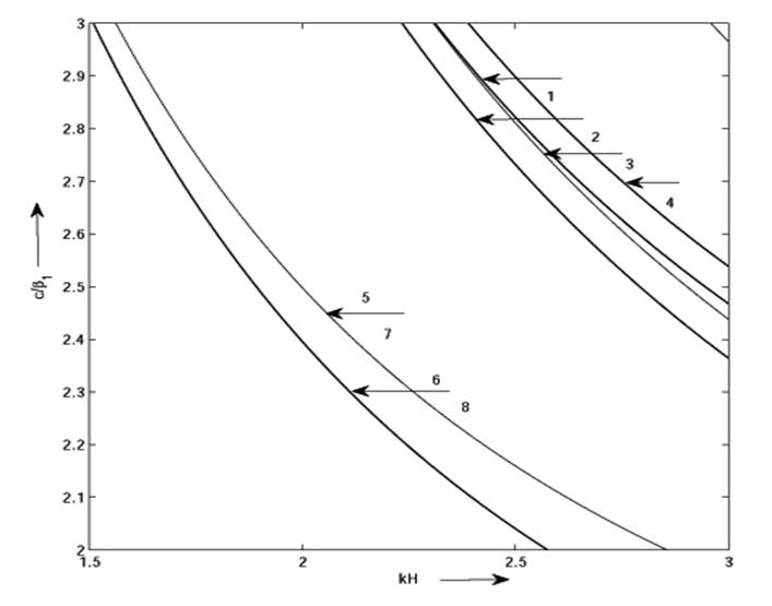
The dispersion curves of Love wave is drawn by taking d=0.6,cc2=0.87,Lμ2=2.5 and other data from Table 1 to Table 5.
Table 1 Parameters of Figure 1
| Rigid Boundary Curve No. |
Traction free Boundary Curve No |
ξ1
|
G
|
| 1 |
5 |
0.3 |
0.3 |
| 2 |
6 |
0.0 |
0.3 |
| 3 |
7 |
0.3 |
0.0 |
| 4 |
8 |
0.0 |
0.0 |
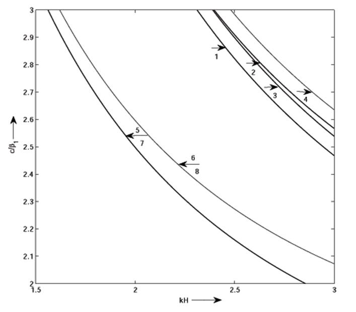
Table 2 Parameters of Figure 2
| Rigid Boundary Curve No. |
Traction free Boundary Curve No. |
ξ1
|
G
|
| 1 |
5 |
0.0 |
0.3 |
| 2 |
6 |
-0.3 |
0.3 |
| 3 |
7 |
0.0 |
0.0 |
| 4 |
8 |
-0.3 |
0.0 |
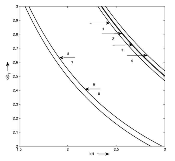
Table 3 Parameters of Figure 3
| Rigid Boundary Curve No. |
Traction free Boundary Curve No. |
G
|
a1k
|
| 1 |
5 |
0.3 |
0.01 |
| 2 |
6 |
0.3 |
0.03 |
| 3 |
7 |
0.0 |
0.01 |
| 4 |
8 |
0.0 |
0.03 |
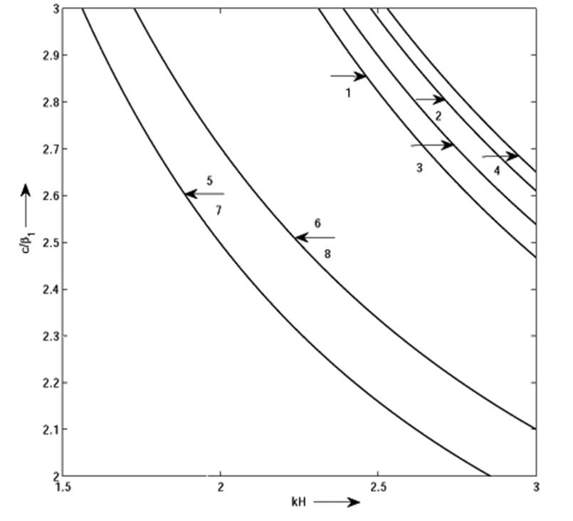
Table 4 Parameters of Figure 4
| Rigid Boundary Curve No. |
Traction free Boundary Curve No. |
ξ2
|
G
|
| 1 |
5 |
0.0 |
0.3 |
| 2 |
6 |
-0.3 |
0.3 |
| 3 |
7 |
0.0 |
0.0 |
| 4 |
8 |
-0.3 |
0.0 |
Table 5 Parameters of Figure 5
| Rigid Boundary Curve No. |
Traction free Boundary Curve No. |
ξ2
|
G
|
| 1 |
5 |
0.0 |
0.3 |
| 2 |
6 |
0.3 |
0.3 |
| 3 |
7 |
0.0 |
0.0 |
| 4 |
8 |
0.3 |
0.0 |
In Figure 1 and Figure 2, the phase velocity of the Love wave in absence of gravity is more than in the presence of gravity in the presence of compressive and tensile initial stress in the upper layer in case of rigid boundary. In case of traction free boundary, the phase velocity of the Love wave is same under the initial stress of the upper layer in the presence or absence of gravity.
The phase velocity of the Love waves in absence of gravity are more than in the presence of gravity without initial stress of the upper layer in rigid boundary, but in case of traction free boundary, the phase velocity of Love wave is same in the presence or absence of gravity without initial stress.
Also we observed that the phase velocity of Love waves in rigid boundary is more than traction free boundary, either upper layer is presence or absence of gravity or initial stress.
In Figure 3, the phase velocity of Love wave in absence of gravity is more than in presence of gravity in presence of heterogeneity parameter in case of rigid boundary where as in traction free boundary, the phase velocity of Love wave is same.
If the heterogeneity parameter increases, the phase velocity of Love wave increases in presence or absence of gravity under rigid where as in traction free boundary the phase velocity decreases.
In Figure 4 and Figure 5, the phase velocity of Love wave in absence of gravity parameter is more than the presence of gravity parameter under compressive and tensile stress in half-space, under rigid boundary, whereas the phase velocity of Love wave is same in case of traction free boundary.
The phase velocity of Love wave in absence of compressive and tensile stress in the half-space is more than the presence of gravity parameter under rigid boundary where as in traction free boundary, the phase velocity of Love wave is same. The phase velocity of Love wave in rigid boundary is always more than the traction free boundary in presence or absence of compressive and tensile stress in the half space.
Conclusions
Propagation of Love waves in porous layer under initially stress over heterogeneous half-space under gravity and initially stress has been investigated analytically in rigid boundary as well as traction free boundary. The dispersion equation is obtained in both the cases. From the figures we may conclude that
In absence or presence of initial stresses in the half-space or layer, the phase velocity of Love waves in rigid boundary is more than the traction free boundary in presence or absence of gravity.
In presence of initial stress in the half-space and absence of initial stress in the layer, the phase velocities of Love wave in traction free boundary is more than the rigid boundary.
Initial stresses play a vital role on the propagation of Love waves in the assumed medium.
Gravity and heterogeneity in the half-space play a notable effect on the propagation of Love waves in the medium and half-space.
Acknowledgement
The authors convey their sincere thanks to Asansol Engineering College, Asansol, Brainware Group of Institutions, Barasat and IIT(ISM), Dhanbad for providing us with its best facility.
The authors are also thankful to the reviewers for their valuable feedbacks about the paper.
References
Abd-alla, A. M. and Ahmed,S. M. ,1999. Propagation of Love waves in a non-homogeneous orthotropic astic layer under initial stress overlying semi-infinite medium. Applied Mathematics and Computation,106(2),449-460.
[ Links ]
Anjana, P.G., Samal, S.K. and Mahanti, S.K, 2010. Love waves in a fluid-saturated porous layer under a rigid boundary and lying over an elastic half-space under gravity. Applied Mathematical Modeling, 34, 1873-1883.
[ Links ]
Biot M.A., 1956, Theory of deformation of a porous viscoelastic anisotropic solid, Journal of Applied Physics 27: 459-467.
[ Links ]
Biot M.A., 1956, Theory of propagation of elastic waves in fluid saturated porous solid, Journal of the Acoustical Society of America 28: 168-178.
[ Links ]
Bacigalupo, A., Gambarotta, L., 2014. Second-gradient homogenized model for wave propagation in heterogeneous periodic media. Int. J. Solids Struct. 51, 1052-1065.
[ Links ]
Chakraborty, M., Chattopadhyay, A. and Dey, S.,1983. The effects of initial stress and irregularity on the propagation of SH-waves. Indian J. pure appl. Math.,14(7),850-863.
[ Links ]
Chakraborty, S.K. and Dey, S., 1981. Love waves in dissipative media under gravity. Garlands Beitragezur Geophysik. 9096 ,521-528.
[ Links ]
Chattaraj, R., Samal, S.K., Mahanti, N., 2013. Dispersion of Love wave propagating in irregular anisotropic porous stratum under initial stress. Int. J. Geomech. 13 (4),402-408.
[ Links ]
Chattopadhyay, A. and Kar, B.K., 1978.On the dispersion curves of Love type waves in an initially stressed crustal layer having an irregular interface. Geophysical Research Bullentin,16(1),13-23.
[ Links ]
Dey, S., Gupta, S., Gupta, A.K., 1996. Propagation of Love waves in heterogeneous crust over a heterogeneous mantle. J. ActaGeophys. Pol. Poland XLIX (2), 125-137.
[ Links ]
Dey, S., Gupta, S., Gupta, A.K., 2004. Propagation of Love waves in an elastic layer with void pores. Sadhana 29, 355-363.
[ Links ]
Gupta, S., Majhi, D.K., Kundu, S., Vishwakarma, S.K., 2013a. Propagation of Love waves in non-homogeneous substratum over initially stressed heterogeneous half-space. Appl. Math. Mech. Engl. Ed. 34 (2), 249-258.
[ Links ]
Gupta, S., Chattopadhyay, A., Majhi, D.K., 2010b. Effect of initial stress on propagation of Love waves in an anisotropic porous layer. J. Solid Mech. 2 (1), 50-62.
[ Links ]
Kalyani, V.K., Sinha, A., Pallavika Chakraborty, S.K., Mahanti, N.C., 2008, Finite difference modeling of seismic wave propagation in monoclinic media. Acta Geophys. 56 (4), 1074-1089.
[ Links ]
Kundu, S., Gupta, S., Manna, S., 2013. SH-type waves dispersion in an isotropic medium sandwiched between an initially stressed orthotropic and heterogeneous semi-infinite media. Meccanica. http://dx.doi.org/10.1007/ s11012-013-9825-5.
[ Links ]
Kundu, S., Gupta, S., Manna, S., 2014. Propagation of Love wave in fiber-reinforced medium lying over an initially stressed orthotropic half-space. Int. J. Numer. Anal. Methods Geomech. http://dx.doi.org/10.1002/nag.2254.
[ Links ]
Manna, S., Kundu, S., Gupta, S., 2013. Love wave propagation in a piezoelectric layer overlying in an inhomogeneous elastic half-space. J. Vib. Control. http://dx.doi.org/10.1177/1077546313513626.
[ Links ]
Pal, P.C., Sen, B., 2011. Disturbance of SH-type waves due to shearing-stress discontinuity in a visco-elastic layered half-space. Int. J. Mech. Solids 6 (2), 176-189.
[ Links ]
Pradhan, A., Samal, S.K., Mahanti, N.C., 2003. The Influence of anisotropy on the Love waves in a self-reinforced medium. Tamkang J. Sci. Eng. 6 (3), 173-178.
[ Links ]
Sharma, M.D., 2004. Wave propagation in a general anisotropic poro-elastic medium with anisotropic permeability: phase velocity and attenuation. Int. J. Solids Struct . 41, 4587-4597.
[ Links ]
Appendix-I
Derivation from equation (2)-(3):
(N-P12)∂2v∂x2+L∂2v∂z2=∂2∂t2ρ11v+ρ12Vㅤandㅤ∂2∂t2ρ12v+ρ22V=0
(2)
Letㅤd2=ρ12v+ρ22V,ㅤthenㅤV=d2-ρ12vρ22
Henceㅤd1=ρ11-ρ122ρ22
Therefore,
(N-P12)∂2v∂x2+L∂2v∂z2=d1∂2v∂t2
(3)
Where, ∂2∂t2ρ12d2ρ22=0, since ρ12d2ρ22 is a constant term.
Appendix -II
Derivation of equation (10):
we have
∂S12∂x+∂S22∂y+∂S23∂z-ρgω23+ρgz∂ω12∂x-ρgz∂ω23∂z-P22∂v∂x2=ρ∂2v2∂t2
(8)
S12=2μexy,S23=2μeyz,eij=12∂ui∂xj+∂uj∂xi,exy=12∂v1∂y+∂v2∂x,eyz=12∂v2∂z+∂v3∂y In this problem ∂∂y=0 and μ=μ21+a1z,ρ=ρ2 , the stress strain relation becomes
exy=12∂v2∂x,eyz=12∂v2∂zS12=μ21+a1z∂v2∂x,S23=μ21+a1z∂v2∂z,∂S12∂x=μ21+a1z∂2v2∂x2∂S23∂x=μ21+a1z∂2v2∂z2+a1μ2∂v2∂z,∂w12∂x=-12∂2v2∂x2,∂w12∂x=12∂2v2∂z2
(9)
where, μ is the modulus of rigidity, a1 is a variation parameter of a rigidity having dimension inverse of length.
Equation (8) using the above relations takes the form
μ21+a1z-12ρ2gz-P22∂2v2∂x2+μ21+a1z-12ρ2gz∂2v2∂z2+a1μ2-12ρ2g∂v2∂z=ρ2∂2v2∂t2(10)


 nueva página del texto (beta)
 Inglés (pdf)
 Artículo en XML
 Referencias del artículo
 Enviar artículo por email
 Citado por SciELO
  Similares en
SciELO
Similares en
SciELO 
 Permalink