


 nova página do texto(beta)
 Inglês (pdf)
 Artigo em XML
 Referências do artigo
 Enviar este artigo por email
 Citado por SciELO
  Similares em
SciELO
Similares em
SciELO 
 Permalink
1 Introduction
The Microsoft Excel calculation memory is one of the basic and universally used tools in engineering and has been enhanced with the inclusion of the Visual Basic language as a programming and task automation tool.
Since its first versions, Visual Basic has allowed the development of several engineering applications due to its ease of learning, simple and immediate implementation, and its versatility that allows the development of programming instructions according to specific needs of the oilwell drilling industry, such as gas correlations, volumetric reserves calculations, simple log analysis, water pattern analysis, among others [17].
The oil industry has undergone a transformation thanks to the advances in computer industry and the introduction of the Internet, which, among other applications, have enabled log acquisition and analysis, reservoir simulation, well testing, production and reserve data analysis, as well as the filling of regulatory reports [7].
Hydraulics plays an important role in many oilfield operations, including drilling, cementing, completion, fracturing, acidizing, production, and reconditioning.
However, in the case of drilling, the role of hydraulics becomes vital, as optimized hydraulics can minimize cost and, conversely, miscalculations can cause problems such as fluid loss, or can even lead to the loss of the well [10].
Drilling is one of the various activities in the oil industry whose main objective is to make a physical connection between the reservoir and the surface.
One of the first computer applications developed was the simulation of a circulation system during drilling; this algorithm had the ability to simulate the washing of the drill string, losing fluid and fracturing the formation [9].
Any hydraulic design developed in well drilling is based on minimizing drilling stresses and reducing associated costs [8]. However, hydraulic modeling is an integral part of the various drilling operations for the realization in an efficient well, the API (American Petroleum Institute) standards consider the Bingham plastic and exponential law models because they provide a simple way to estimate the necessary parameters for efficient drilling of conventional wells [18].
The importance of optimizing drilling fluid properties lies in ensuring drilling operations and process safety [14]. In consideration, the evaluation and prediction of well cleanliness presents a challenge in the drilling industry, since good well cleanliness means a high penetration rate and fewer drilling problems [1].
Additionally, it has been observed that drilling fluids with similar properties according to the API standard can have significantly different behavior with respect to cuttings transport efficiency, resulting this in a research topic in recent years [15].
Still, nowadays these properties are manually measured and optimized by engineers with different skills and experiences that at a certain moment could lead to non-optimal characteristics of the drilling fluid, i.e., cause a deterioration of its functionalities.
To minimize these events, the use of software would allow the study of various scenarios that could be supported by the experiences of design and operating engineers, especially when wellbore cleanliness and stability conditions change during drilling.
One of the areas of opportunity in the study plans and programs of technical and university bachelor’s degrees related to petroleum engineering is the lack of simulation software, that allows the development of design and analysis skills for well drilling and fluid exploitation processes in accordance with relevant technical standards and engineering practice.
On the contrary, several national and international oil sector companies have developed their own computational models that are restricted for use by their personnel or are commercially available at prohibitive license costs that are unaffordable for higher education institutions.
In addition, well drilling fluid hydraulics software represents, within the teaching-learning process, a considerable reduction of time compared to manual calculations, thus giving the opportunity to perform a greater number of design simulations and the consequent analysis of alternatives in oil well drilling.
The objective of the present work was to develop a computational model in the Microsoft Visual Basic environment whose purpose is to simulate and optimize the hydraulic processes related to onshore oil well drilling.
This model considers two rheological models (Bingham plastic and exponential law) to comprehensively simulate variable rheological behavior, as reported in technical literature [3]; that is, a drilling fluid rheology could match a model behavior at the surface and act as another fluid downhole.
Some studies have revealed that mud rheology, density, transport velocity, tubing rotation and well depth are the controlling factors that influence wellbore cleanup [5]. The model presented here meets a series of desirable technical considerations, such as: i) ease of use, ii) simulation options in line with real operational activities, iii) accurate and validated calculations, iv) unnecessary periodic software updates, v) use of the software without the need for technical support, and vi) low memory space requirements and compatibility with Excel 2010 and later.
Likewise, this software brings together valuable academic aspects since it allows: i) technical training for inexperienced professionals, ii) problem-based learning for technical and university degree students, and iii) the use of two well hydraulics methodologies and two rheological models.
2 Methodology
Drilling engineering is very complex, so much so that the design of a program contains so many important variables of study ranging from the physicochemical composition of a fluid, casing selection and setting, drill string design, bit types and surface connections, to name a few.
Four sections were developed for this program: I) Cover, II) Hydraulics I, III) Hydraulics II, and IV) Rheological Models.
2.1 Cover
Cover section is integrated by basic information of the well, such as name, number, classification, objectives, and geographic coordinates of the well.
These data are part of the design or user’s guide used by Petróleos Mexicanos for each of its drilling projects, which is considered a standard in the presentation of projects for service companies. Likewise, this section is complemented by a subsection that welcomes the user and briefly describes the content of the software and its procedures or hydraulic methods, in addition to indicating the technical literature used for its development.
2.2 Hydraulics I
Hydraulics I section is mainly developed by the methodology described by Petróleos Mexicanos (Pemex), [11, 12, 13]. Due to the experience in the field and in trainings by active personnel in the area of oil well drilling, all the above, is integrated as shown in the flow chart shown in Figure 1.

Hydraulics I calculations require entering casing and drillstring information such as initial and final lengths (
In this regard, the typical grades, from lowest to highest strength, are
Once the mechanical state is appropriate, the program requests information on: i) The drilling fluid: density (
where
In general, the drillstring is composed of three types of pipes: drill collar, heavy weight and drill pipe. In particular, drill pipe has two subtypes: new pipe and (premium) used pipe. The calculation procedure determines the design of the drillstring and casing.
From this design, the number of sections, the annular volume (
Furthermore, the adjusted weight (
2.3 Hydraulics II
Similarly, the Hydraulics II section is based on a combination of the methodologies described in [4]. Field experience and training material from international companies, which can be found in the flow chart in Figure 2.

2.4 Rheological Models
Finally, the section Rheological Models is integrated by the results of the Fann viscometer test with which rheology values are calculated for low and high shear rate using the Bingham plastic and exponential law models [6].
Drilling fluid hydraulics refers to the fluid that performs a path that starts its displacement by means of mud pumps, which can be duplex or triplex, which are considered the heart of the circulatory system and that concludes in the settlement dam.
For the realization of the program, it was necessary to know the diagram or fluid circulation circuit during the drilling or circulation stages, as shown in Figure 4. The flow diagram of the calculation processes allows to identify the sections and the sequence of the programming, which have the following order:
Schematize the diameters and depths of the casing pipes or casing.
Draw the pipes with diameters and depths that integrate the drill string. Establish the minimum necessary information such as: mud pump characteristics, drilling fluid type and density, fluid rheology, drill cuttings characteristics and types of connections.
Corroborate that the annular spaces and string interior correspond to the mechanical condition (MS) design.
Relate input data to annular volumetry and string interior calculations.
Identify the possible cases according to the MS design.
Develop the hydraulic method according to the input data.
Apply the Fann viscometer test values in the rheological models.


In the applied hydraulics calculation procedure, the flow rate and string consistency parameters (
On the other hand, the consistency index is considered as plastic viscosity, either by an increase in the concentration of solids or a decrease in the particle size.
Its control is achieved with mechanical solids control and dilution equipment. Additionally, these indices are also calculated for the annular space, denoted as
Additionally, the calculations of average propagation velocity, effective viscosity, Reynolds number, Fanning friction factor and pressure loss are determined for each of the drillstring and annular space interior volumes generated from the mechanical state design.
The friction factor is determined by considering the value of the Reynolds number (
Depending on whether the flow regime is predominantly laminar or turbulent, the friction factor (
where
The calculations in the Complementary Hydraulic Calculations section correspond to drilling optimization, i.e., estimating a penetration rate according to bit performance [4], since among the many factors that can modify it are, for example:
Bit size, type and characteristics, type and concentration of solids in the formation, and bit hydraulics. However, the latter can be optimized by controlling hydraulic power and nozzle velocity.
3 Results
Application Examples
To demonstrate the capabilities of the software, two illustrative examples of oil well drilling have been selected. First, a calculation procedure using the national methodology and, subsequently, an exercise developed under the API methodology.
Introduction Section and Description of Hydraulics
Figure 3 corresponds to the front page of the software, which requests basic information from the design guide, in order to know the name, number, location and objective of the well, as well as the name of the technician or design engineer.
To perform the first hydraulic calculations, it is required to enter a set of data whose information is classified into seven elements: casing, borehole, drillstring, pump, mud properties, nozzles and cuttings.
Table 1 provides the necessary information to exemplify the use of this tool using national petroleum engineering methods and procedures.
Table 1 Initial information required by the program (national methodology)
| Element | Dimensions and Properties | |||||
| Casing Pipe |
|
Depth |
||||
| Driven | 29 | 150 | ||||
| Superficial | 23 | 600 | ||||
| Intermediate | 17 | 1,200 | ||||
| Explotation | 11 | 2,100 | ||||
| Borehole | 9 | 2,100 – 2,500 | ||||
| Drillstring |
|
|
|
|
||
| Drill collar | 7 | 2.25 | 2,500 – 3,000 | 136 | ||
| Heavy weight | 5 | 3.00 | 2,300 – 2,200 | 74.5 | ||
| Drill pipe | ||||||
| Section | Degree |
|
|
|
|
|
| Tp1 | 127,181 | 4 | 3.00 | 2,200 – 900 | 31.12 | |
| Tp2 | 161,096 | 4 | 3.00 | 900 – 300 | 31.94 | |
| Tp3 | 178,054 | 4 | 3.00 | 300 | 32.66 | |
| Pump (triplex type) |
|
|
|
|
||
| 6.5 | 12 | 90 | 105 | |||
| Fluid Properties |
|
|
|
|
||
| 1650 | 0.1 | 24 | 22.7 | |||
| Nozzels |
|
|||||
| 3 | 16/32 | |||||
| Cuttings | Lenght (cm) | Width (cm) | Thickness (cm) | |||
| Dimensions | 4 | 3 | 3 | |||
| Density (kg/m3) | 2,700 | |||||
| Other Dimensions | ||||||
| Steel density (kg/m3) | 7,850 | |||||
| Total depth (m) | 2,500 | |||||
| Surface pressure (kPa) | 345 (50 psi) | |||||
| Bit diameter (in) | 9 in | |||||
Technical Data and Mechanical State Section
Figure 5 corresponds to the input of technical data of the casing pipes, drillstring, mud pumps, bits, solids/cuttings and the drilling fluid whose first result corresponds to the generation of the mechanical state, in which it can be identified the number of annular spaces both in the hole section and in the casing pipes.
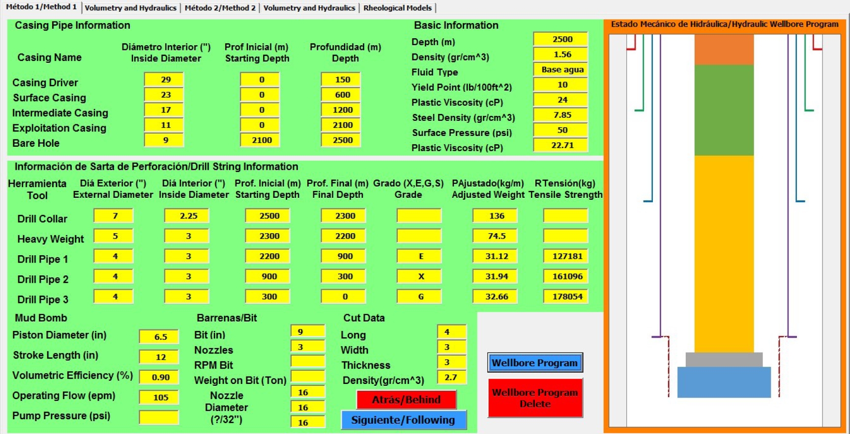
The drillstring is outlined with a color code: the blue color is the drill collar, the gray color is the heavy weight, and the orange, green and brown colors correspond to the drill pipes in the order Tp1, Tp2 and Tp3, respectively.
It is important that the design engineer or technician corroborate the MS schematic in this section as it determines the volume of drilling fluids inside the string and the corresponding hole sections, casing pipes, and drillstring tools.
Hydraulics I Section
Figure 6 begins with the evaluation of the drill pipes (Tp), the pull margin, the flotation factor, and the weight of the floating drillstring.

Fig. 6 Results of: string design, annular and optimal velocity, interior volume, circulation times and system pressure
Subsequently, the calculations according to the MS design are obtained, such as: hole-string annular volumetry, internal volume of each of the tools that make up the drillstring, expenses and circulation times, annular and optimal speeds, speed and area of nozzles, internal pressure in the drillstring, hydraulic parameters, pressure in annular intervals, transport of cuttings, among others.
Each of the previous points has its respective physical units and four decimal places of precision, as shown in Table 2.
Table 2 Results of hydraulic calculations using the national methodology
| Result | Value |
| Drill pipe position evaluation | |
| Flotation factor (-) | 0.8013 |
| String weight (kg) | |
| Floated | 83,391 |
| 1: Tp1-Tp2-Tp3 | 43,791 |
| 2: Tp2-Tp3-Tp1 | 77,706 |
| 3: Tp3-Tp2-Tp1 | 94,664 |
| Determination of volumetries, times and speeds | |
|
|
121,101.3 |
|
|
11,001.7 |
| Pump expense (L/min) | 1,850.5 |
| Circulation Times (min) | |
| Time of delay | 65.4 |
| Full cycle time | 136.8 |
| Travel time | 71.4 |
| Annular velocities, |
|
| Ag-DC | 114.1 |
| Ag-HW | 65.2 |
| Ag-Tp1 | 56.2 |
| TR-Tp1 | 34.8 |
| Optimal velocities, |
|
| Ag-HTA | 100.9 |
| TR-HTA | 82.5 |
| Determination of pressure drops and cutting speed | |
| Nozzle area (in2) | 0.5890 |
|
|
824.7 (58 kg/cm2) |
|
|
4,441.8 (312 kg/cm2) |
|
|
64.4 (4.5 kg/cm2) |
|
|
278.4 (4.6 m/s) |
| Fluid Carrying Efficiency (%) | 78 |
Accurate estimation of pressure drop is important for the design of the drillstring, nozzles and for optimizing fluid circulations, as well as identifying drilling problems such as flushing or clogging of the bit nozzles [2].
Hydraulics II Section
To illustrate the use of the Hydraulics II Section, referring to the hydraulic methodology established in [6], the data will be entered as shown in Figure 7.
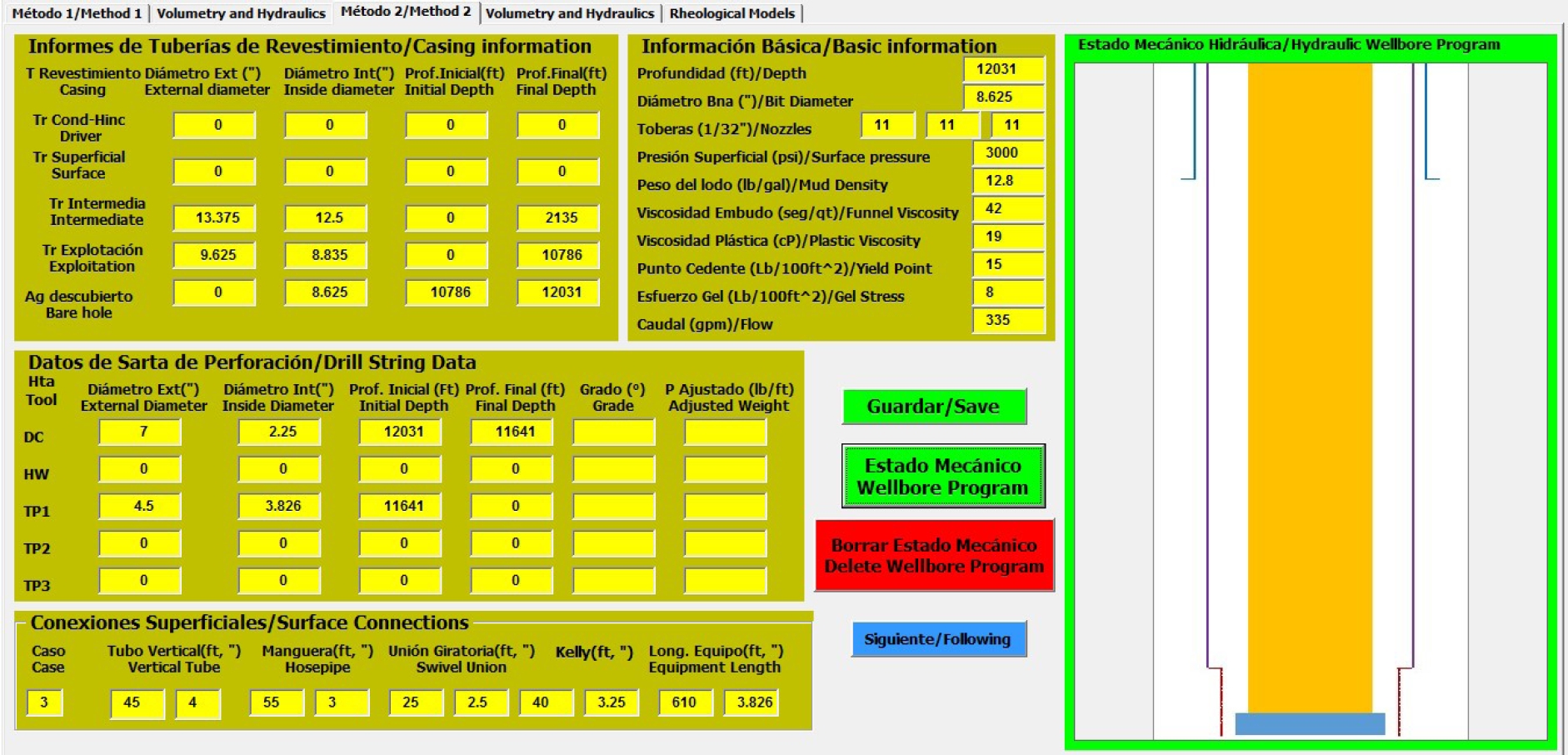
This methodology is used by transnational oil companies, the information indicated in Table 3 is required. The exercise used corresponds to the example of the API manual.
Table 3 Information required by the program (API methodology)
| Element | Dimensions and properties | ||||
| Casing Pipe |
|
|
Depth |
||
| Intermediate | 13.375 | 12.500 | 2,135 | ||
| Exploitation | 9.625 | 8.835 | 10,786 | ||
| Drill string | |||||
| Hole | 8.625 | 10,786 – 12,031 | |||
| Drill collar | 7.000 | 2.250 | 12,031 – 11,641 | ||
| TP1 | 4.500 | 3.826 | 11,641 | ||
| Surface connection (case 3) |
|
Length (ft) | |||
| Vertical Pipe | 4.00 | 45 | |||
| Hose | 3.00 | 55 | |||
| Swivel joint | 2.50 | 25 | |||
| Kelly device | 3.25 | 40 | |||
| Equipment length | 3.82 | 610 | |||
| Nozzles |
|
||||
| 3 | 11/32 | ||||
| Fluid properties |
|
|
|
|
|
| 12.8 | 0.15 | 0.08 | 19 | 42 | |
| Other dimensions | |||||
| Total depth (ft) | 12,031 | ||||
| Surface pressure (psi) | 3,000 | ||||
| Bit diameter (in) | 8.625 | ||||
For this procedure it is required to know the results of the Fann viscometer tests and the value of the total pressure of the surface system, and to identify the corresponding case of the types of surface connections with which the drilling equipment is operating.
Figure 7 right, schematizes the mechanical state according to the data of the various casing pipes and tools that make up the drillstring. Figure 8 shows the solution of the exercise.

Figure 8 corresponds to the results of the applied hydraulics operations, where initially the readings are determined at different rotational speeds of the viscometer, i.e. 600, 300, 100, and 3 rpm, where the lowest speed corresponds to a low shear stress.
From these data, the flow and consistency indices of both the string and the annular space (
Once the type of surface connection is identified, it is essential to know that it is integrated by the vertical pipe, the kelly device hose, swivel joint and the kelly ”traveling rotary”; but as there is no standard value for the traveling rotary it is important to know the geometry of each of them, for example, the vertical pipe and hose measure approximately
The resulting hydraulic calculations are summarized in Table 4. After the mechanical state is generated, the Fann viscometer readings are entered to determine the
Table 4 Hydraulic calculation results using API methodology
| Result | Value | ||
| Rheological parameters | String | Annular space | |
| Flow index |
0.64 | 0.26 | |
| Consistency index |
3.20 | 26.46 | |
| Fann Viscometer readings | |||
| @ 600 rpm | 53 | ||
| @ 300 rpm | 34 | ||
| @ 100 rpm | 23.1 | ||
| @ 3 rpm | 8 | ||
| Variables of surface connections | |||
| Propagation speed (ft/min) | 560.23 | ||
| Effective viscosity (cP) | 48.98 | ||
| 8,663 | |||
| 0.0060 | |||
| Surface connection pressure (psi) | 41.54 | ||
| Drillstring variables | Drill collar | Tp-1 | |
| Propagation speed (ft/min) | 1619.91 | 560.23 | |
| Effective viscosity (cP) | 27.61 | 48.98 | |
| 26,133 | 8,663 | ||
| 0.0044 | 0.0060 | ||
| Pressure (psi) | 277.9 | 792.8 | |
| Variables for annular sections | Ag-DC | Ag-TP | TR-TP |
| Propagation speed (ft/min) | 322.98 151.47 | 141.86 | |
| Effective viscosity (cP) | 34.15 | 117.86 | 128.24 |
| 3,042 | 1,049.5 | 949 | |
| 0.0047 | 0.0229 | 0.0253 | |
| Pressure (psi) | 16.1 | 15.0 | 174.4 |
Finally, to complete the hydraulic design of the well, and regardless of the number of sections and the type of pipe to be used, it is essential to perform complementary calculations, which are summarized in Table 5.
Rheological Models Section
Figure 9 corresponds to the Rheological Models Section, which allow describing the relationship between shear stress and shear velocity. Most drilling fluids are non-Newtonian fluids, which is why Newton’s viscosity law or model does not describe their flow behavior. For this program, the Bingham plastic and exponential law models were implemented.

In recent years, the Bingham plastic flow model has been one of the most widely used to describe the flow characteristics of drilling fluids; however, this model is characterized by requiring a finite force to initiate the flow to subsequently develop a constant viscosity as the shear rate increases.
The curve or profile of a typical or conventional fluid is obtained from the rotary viscometer data, where this curve does not pass through the origin point, as shown in the graphs in Figure 9 and Figure 11, between shear rate and shear stress.
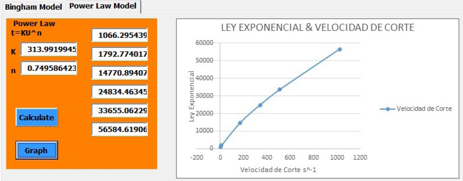

In Figure 10, the exponential law model does not assume that there is a linear relationship between shear stress and shear rate; however, for fluids obeying the exponential law, its curve starts from the origin.
In this model it is confirmed that the shear rate varies according to the change in shear stress. The Bingham rheological and exponential law models are among the most used and important for the determination of pressure loss in the drilling system [16].
Finally, for the Hydraulics II section, the value of

Fig. 12 Effect of Exponential Law index n on velocity profile. Adapted from API Energy Handbook (2001)
Nevertheless, if the value of
In addition, this methodology allows to contrast the result with the initial surface pressure value, allowing to know more quickly if the applied hydraulics is in accordance with what the surface monitoring equipment indicates.
4 Conclusions
The computer model developed in the Microsoft Visual Basic environment is an efficient and useful tool for the calculation of various hydraulic aspects related to oil well drilling. The interface design is simple and intuitive, of fast communication and easy adaptation between program and user.
The computer program integrates two hydraulic methodologies in a didactic way, but keeping in each of them its originality, development philosophy and in accordance with the field operation. In the program, the existing theory in the specialized literature is combined.
The mechanical state schematization considers the scaled relationships of casing and drillstring dimensions, and knowledge of the mechanical state is essential for consideration, analysis and interpretation of hydraulic methods.
In the future, this model will be enhanced to allow the user to make custom modifications based on their experience or internal company design criteria; for example, propose bit, annular space or drillstring pressure drops, or modify nozzle diameters and make adjustments based on the maximum hydraulic power or maximum hydraulic impact method.
Additionally, this computer program considers the two most commonly used rheological models, although in a later version new models will be included so that the user has greater flexibility according to the information available in his design project.
This tool aspires to become the most widely used software in higher education institutions where new technicians and engineers are trained, as well as a support tool in training courses for the oil well drilling industry.

