Ensemble spread and systematic errors in the medium–range predictions during the Indian summer monsoon

 

S. C. KAR, G. R. IYENGAR and A. K. BOHRA
National Centre for Medium Range Weather Forecasting, A–50, Sector–62, NOIDA, India 201307. Corresponding author: S. C. Kar; e–mail: sckar@ncmrwf.gov.in

 

Received October 2, 2008; Accepted August 26, 2010

 

RESUMEN

En el National Centre for Medium Range Weather Forcasting (NCMRWF) de la India se utilizan dos modelos globales, a diferentes resoluciones, para preparar pronósticos de tiempo de rango medio. Para mejorar la habilidad de los pronósticos se implementó, de manera experimental, un sistema ensamblado de predicción (EPS). Se realizaron corridas de pronósticos experimentales con un ensamble de ocho miembros y los resultados se analizan para la temporada del monzón. La media de los pronósticos de precipitación del ensamble muestra que, sobre una amplia región de las planicies del Ganges, el EPS muestra la actividad del monzón (activo y débil) de manera razonablemente buena con un avance de hasta seis días. Sin embargo, en las partes orientales de la India la media de precipitación del ensamble es buena sólo en rango corto. La propagación del ensamble se hace bastante grande a partir del día 4 del pronóstico y más allá. El examen del patrón de precipitación del modelo y de la propagación del ensamble, para los días 1 a 6 de pronóstico, muestra que no hay relación lineal entre el incremento de la propagación y la cantidad de precipitación. El modelo tiene la tendencia sistemática de incrementar la actividad de precipitación sobre la parte central de la Bahía de Bengala y las partes orientales de la India al incrementarse la longitud del pronóstico. Al mismo tiempo el modelo tiende a secar la región ecuatorial del Océano Índico, sin embargo esta tendencia no se observa en el modelo de alta resolución. En los campos de circulación el modelo también tiene errores sistemáticos grandes. Los resultados sugieren que para obtener el máximo beneficio del EPS las desviaciones sistemáticas del modelo deben reducirse ya que el método de anidamiento considera únicamente las incertidumbres de las condiciones iniciales y no los errores relacionados con el modelo.

 

ABSTRACT

For preparing medium range weather forecasts, two global coarse resolution models at different resolutions were used at the National Centre for Medium Range Weather Forecasting (NCMRWF), India. In order to improve the forecasting skill, an ensemble prediction system (EPS) was implemented on experimental basis. For generating initial perturbations a breeding method was implemented. Experimental forecast runs with 8–member ensemble were carried out and results are analyzed for a monsoon season. The ensemble mean of rainfall forecasts shows that over the broad region of Gangetic Plains, the EPS brings out the monsoon activity (active and weak spell) reasonably well six days in advance. However, over the eastern parts of India, the ensemble mean rainfall is good only in short–range. The ensemble spread becomes quite large from about day–4 forecast and beyond. An examination of the rainfall pattern from day–1 to day–6 forecasts by the model and the ensemble spread shows there is no linearity in the increase of spread with the rainfall amount. The model has a systematic tendency to enhance rainfall activity over the central Bay of Bengal and eastern parts of India as the length of forecast is increased. At the same time, the model tends to dry up over the equatorial Indian Ocean region, however, in the high–resolution model, the same tendency is not seen. In circulation fields, the model also has large systematic errors. These results suggest that to obtain maximum benefit from the ensemble prediction system, the systematic biases in the model must be reduced as the breeding method only takes care of the uncertainties in the initial conditions.

Keywords: Forecast, rainfall, skill, spread, global, model.

 

1. Introduction

Prediction of the Indian summer monsoon rainfall in short– and medium–range timescale is quite important for the economy in the Indian subcontinent as it is largely dependent on agriculture. Success or failure of the crops and water scarcity in any year is always closely linked with the amount of the monsoon rains received in India (Kumar et al., 2004). While the India Meteorological Department (IMD) was responsible for providing operational seasonal monsoon prediction and short–range (1–2 days in advance) weather forecasting to the public in India, the National Centre for Medium Range Weather Forecasting (NCMRWF) was established to prepare and disseminate medium–range (3–10 days in advance) weather forecasts for agro–meteorological applications. For this purpose, NCMRWF had established more than 100 field units across India, and they routinely receive the weather forecasts and prepare agro–meteorological advisories for the farming community, (Rathore and Maini, 2008).

Short– and medium–range predictions of rainfall over any region, including that over the Indian region during the monsoon season depend on how well the initial state of the atmosphere has been defined with large number of very good quality observed data and the quality of dynamic models used for prediction. The better the initial data, better is the forecast. Similarly if the model used is more detailed and contains state of the art schemes to describe atmospheric physics and dynamics, forecasts from this model shall be better. However, there is a limit to which one can make usable predictions. In the tropical region, the predictability of day–to–day weather is restricted to 3–4 days (Mani et al., 2009). Scientists are engaged to extend this limit of predictability. Deterministic predictability as such cannot be extended, but predictability of weather systems, weather types, flow regimes, etc. can be extended further. The atmosphere is a chaotic system, and as a result, small errors in our estimate of the current state can grow to have a major impact on the subsequent forecast. Because of the limited number of observations available and the uneven spread of these observing platforms around the globe, there will always remain some uncertainty in the estimate of the current state of the atmosphere.

Ensemble forecasting method is based on the recognition of above facts that any error in initial conditions or model formulation shall lead to loss of predictability after a finite period of time (Toth and Kalnay,1997). Several numerical modeling experiments have also shown that, predictability greatly varies in time and space depending on the flow in the atmosphere. The objective of ensemble forecasting is to identify these flow dependent variations in advance, and incorporate these in the forecasting method. Ensemble forecasting method entails running of a numerical weather prediction (NWP) model (or several model variants) a number of times, with slightly perturbed initial conditions, to assess the forecast uncertainty due to errors in the initial conditions and possibly in model formulation. These methods are routinely used at major operational NWP centers around the world: European Centre for Medium Range Weather Forecasts (ECMWF) (Leutbecher and Palmer, 2008), National Centers for Environmental prediction (NCEP), (Toth and Kalnay, 1997); the Canadian Meteorological Center (CMC) (Houtekamer et al., 1996), the Japan Meteorological Agency (JMA) (Kobayashi et al., 1996).

Toth and Kalnay (1993, 1997) introduced the breeding technique that identifies those possible analysis errors that can amplify most rapidly. Singular vectors technique (Molteni et al., 1996) identifies perturbation structures that can grow fastest in the forecasts. There are different attempts to account for model related uncertainty in ensemble forecasting. Houtekamer et al. (1996) and Houtekamer and Lefaivre (1997) have taken this into account by running several versions of an NWP model in parallel with each other. These versions differ from each other in horizontal resolution, treatment of orography, convection and radiation parameterization, etc. At ECMWF, after each time step within a model integration, stochastic multiplicative noise was added to the diabatic forcing term. After the forcing from all parameterized processes is added up, the net forcing is multiplied by a number chosen randomly, making the impact of the complete physics package stochastic (Buizza et al., 1999). The goal is to represent the inherent uncertainty in the parameterization of subgrid–scale processes that leads to the emergence of stochastic errors during model integrations.

Prediction of the Indian summer monsoon rainfall in medium–range has remained a challenging problem. There are large uncertainties in initial conditions over the Indian monsoon region, as India is surrounded by vast oceans (Arabian Sea, Bay of Bengal and the Indian Ocean). The Himalayas to the north of India is also a data sparse region. Therefore, the observations available to define the initial conditions for a numerical model may not be adequate. A large number of observations are available in recent years from satellite based sensors. However, there are several issues regarding the quality of data available from them, the retrieval methods used, and calibration procedures involved over the Indian region (Kar et al., 2003). There is always some scope for improvement in prediction methods and predictions. Use of better/denser observing networks to determine small scale structures in the initial conditions could benefit the prediction at synoptic and perhaps sub–seasonal lead times.

The NCMRWF has been a lead center in India for all weather and climate model related research, where an operation and real–time global and regional data assimilation works are being carried out for providing operational medium–range weather forecasting. Global models and data assimilation systems atT170L28 and T80L18 resolutions were run routinely forproviding operational weather forecasts. Recently the global model resolution has been further enhanced. So far, weather forecasts at the Centre are based on the direct model output of these models and their statistical interpretation. All the model runs begin with initial conditions at 0000UTC of the day and 7–day forecasts are made. However, no runs are made on operational basis with perturbations to initial conditions for having a set of ensemble forecasts. Considering the fact that there are large uncertainties in the initial conditions, especially over the Indian domain, it was proposed to implement an Ensemble Prediction System (EPS). It is believed that the EPS can be used as a quantitative tool for risk assessment in a wide range of weather–sensitive commercial and humanitarian activities. The potential economic value of the EPS can be much higher than that of a forecasting system based on only a single deterministic forecast (e.g. Richardson, 2000; Zhu et al., 2002).

The main objective of this study is to describe the EPS implemented at NCMRWF, to document the results of several forecast runs from the EPS, and to describe the spread of ensemble forecasts and relate them to the model systematic errors. Section 2 of the paper describes the forecasting system, the models used in EPS as well as the breeding method used to generate the perturbations. In Section 3, results of model forecasts from the EPS are presented and discussed. In Section 4, the study is concluded.

 

2. The NCMRWF forecasting system and the ensemble method

2.1 The assimilation method and the models

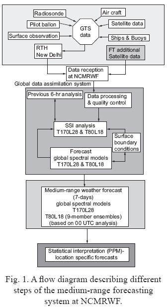
At the NCMRWF all the observation data through Global Telecommunication System (GTS) are received in real–time as half–hourly files. In addition, data from several satellites (non–GTS data) are downloaded in real–time through Internet. A 3–dimensional variational analysis system based on Spectral Statistical Interpolation (SSI) technique (Parrish and Derber, 1992) is used to carry out a consistent atmospheric analysis. The data assimilation is done at a 6–hour cycle. Two different global spectral models are run. The models have triangular truncation with T170 waves in the horizontal and 28 vertical layers (T170L28), and T80 waves in the horizontal and 18 vertical layers (T80L18). The T170L28 model was developed at NCMRWF and is described in Kar (2002). The main time integration scheme is leapfrog for nonlinear advection terms, and semi–implicit for gravity waves and for zonal advection of vorticity and moisture. The time step is 15 minutes for the T80L18 model, and 7.5 minutes forthe T170L28 model for computation of dynamics and physics, except that the full calculation of long wave and shortwave radiation is done once every six hours. Deep convection is modeled by a fairly basic Kuo–Anthes type of scheme, requiring moisture convergence and deep conditional instability in order to be active (Kuo, 1974; Anthes, 1977). Soil temperature and soil volumetric water content are computed in two layers (Pan and Mahrt, 1987). The lowest model layer is assumed to be the surface layer and the Monin–Obukhov similarity profile relationship is applied to obtain the surface stress and sensible and latent heat fluxes. Above the surface layer, a first order non–local closure assumption is made to distribute the fluxes in the planetary boundary layer (Hong and Pan, 1996; Basu et al., 2002). More details of the model may be found at Kanamitsu et al. (1991), and Kar et al. (2002). The models at both resolutions are run starting with 0000 UTC of each day and are run for preparing 7–day forecasts. A flow diagram schematically describing different steps of the forecasting system is shown in Figure 1. Recently, this forecasting system has been upgraded by using a global model at T254L64 resolution from NCEP, USA.

2.2 Ensemble method

The ensemble forecasting at the Centre involves the integration of the operational NWP model with several perturbed initial conditions. In this method, the control analysis is taken as the best estimate of the truth. Perturbations are estimated as representative of the errors in analysis. The numerical model from these perturbed analyses is integrated and forecasts are interpreted. The breeding of growing modes method (Toth and Kalnay, 1993) has been implemented as a part of the EPS system at the Centre. In this method, very small perturbation to the analysis (initial state) at a given day to is added and subtracted. The difference between an analyzed field and model's first guess (6–hour forecast) was chosen as the initial perturbation. Then the model is integrated from both the positively and negatively perturbed initial conditions for one day. One forecast from the other is subtracted. Then the difference field is scaled down so that it has the same norm (e.g. root mean square of kinetic energy) as the initial perturbation. Then the difference obtained is added to the analysis of the next day. At the Center, the ensemble prediction system is implemented at the T80L18 resolution. We allowed the bred vectors to develop before using them. This was achieved by running the ensemble scheme for one more season prior to the period of analysis. Number of ensemble members are eight, in addition to a control run which does not have any perturbation. Though the number of ensemble members is not large in this study, it is hoped that if significant improvement is obtained in the forecasts using the EPS based on a cost–benefit analysis, the number of ensemble members shall be further increased.

2.3 Modeling experiments using EPS

After implementation of the EPS system based on the T80L18 model using the breeding cycle procedure, the EPS was run to prepare medium–range weather forecasts for the entire monsoon seasons (from June 1 to September 30) of 2005. Year 2005 was chosen because it was a normal monsoon year and there were identifiable active and break phases of the monsoon during the season. Therefore, this season was suitable to check the characteristics of monsoon prediction in medium–range timescale using the ensemble prediction scheme. The T170L28 model runs provided the single high–resolution forecasts. Control runs were made using the T80L18 model with the operational analysis as initial conditions. Eight numbers of perturbed analysis were prepared which were used as eight more initial conditions. Ensemble mean of all the forecasts were prepared and examined along with the high–resolution model runs. The real–time global analyses prepared at the Centre were used to verify the forecasts of atmosphere. The gridded rainfall analysis prepared by IMD (Rajeevan et al., 2006) was used for verifying the rainfall forecasts over the Indian region.

 

3. Results and discussion

3.1 Monsoon season–2005

Before describing the results of the EPS, the monsoon season of 2005 is briefly described. The mean analyzed wind field for June, July, August and September (JJAS), 2005 at 850 hPa level is shown in Figure 2a. The important semi–permanent circulation features of the monsoon flow over the Indian subcontinent, namely the cross–equatorial flow over the Arabian Sea and the associated low level jet, and the monsoon easterlies over the Gangetic Plains, are of the analysis. At the 200 hPa, the tropical easterly jet is visible and the Tibetan anticyclone is at about 90E and 29N, its normal position (not shown in figure). Figure 2b shows the wind anomalies at 850hPa for JJAS 2005. The anomalies are computed based on climatology of last 14 years of the NCMRWF analysis. An anomalous cyclonic circulation is seen over the south Arabian Sea, which weakens the monsoon winds over the south west coast. Cyclonic anomalies are found to have prevailed over the north–western region, and westerly anomalies are seen in the plains of north India and north eastern parts of the country leading to subdued rainfall activity over this region. There are anomalous north easterlies over the Bay of Bengal which turn to easterlies near the east coast of India and prevail over most part of central India. Over the equatorial Indian Ocean, a zonal band of anomalous westerly winds is seen, which carry away a part of cross equatorial wind from the Somalia coast.

The observed rainfall during the monsoon season of 2005 from IMD is shown in Figure 2c. The observed rainfall data are station and rain gauge merged data gridded to regular 1X1°. As is well known, the Indian monsoon is characterized by zones of maxima in rainfall during the season. Over the west coast, there is a maxima in rainfall with more than 20 mm/day in the seasonal mean. Day to day variations of rainfall in this region are quite large, and occasionally rainfall of about 30–40 cm/day is also received in this region. It may be noted that in July 2005, Mumbai received a record of 94 cm during a single day. However, when data is averaged to make a 1x1° gridded set, rainfall of such magnitude is not noticed. The eastern and east–central parts of India is another region in which a maxima of rainfall is seen during monsoon season of 2005. Large interannual and intraseasonal variations of rainfall during a monsoon season are observed in this region. Monsoon lows and depressions form over the Bay of Bengal during the season, and travel to Indian subcontinent passing over this region. During 2005 monsoon season, this region received about 8–16 mm/day rainfall as seen in the figure. Figure 2d shows the observed rainfall anomalies for JJAS 2005, computed on the basis of observed rainfall data described in Rajeevan et al. (2006). The dataset covers from 1951 to 2003, based on which the climatology has been prepared. Due to a cyclonic anomaly off the west coast of India, this region received more rain than normal during this season. The maximum positive anomaly is seen around the western coast which is 8–12 mm/ day more than normal. Regions surrounding eastern and north–east India received less than normal rainfall during this season. The central region of the country received good amount of rainfall in this particular season as compared to climatology of the region.

3.2 Modeling results

Figure 3a shows averaged rainfall forecasts of all day–4 (96–hours) for JJAS 2005 obtained from data assimilation forecast system at T170L28 resolution. Figure 3b shows the same plot for the rainfall forecasts of the control runs at T80L18 resolution. For describing seasonal averaged rainfall forecasts, day–4 has been chosen as day–1 to day–3 rainfall may have errors due to spin–up and longer range forecasts may have been degraded due to systematic errors. Agreeing very well with observation, the T170 model predicts about 16–20 mm/day or more over the Western Ghat region. The model also predicts about 12–16 mm/day rainfall over the eastern and the central parts of India. The model predicted rainfall over the foothills of Himalayas can not be compared with any observations as the observed data available from IMD is only over India. Nevertheless, the high–resolution model brings out major rainfall zones as observed during the season in day–4 forecasts. An analysis of rainfall forecasts from other days also shows very similar features. The coarse resolution global model at T80 resolution broadly brings out the essential features of the rainfall distribution during the monsoon season under consideration. However, the magnitude of rainfall predicted is too low. Over the west coast of India, the model predicts a broad region of 12 mm/day rainfall. Over the eastern parts of India, the model predicts only about 8–12 mm/day of rainfall. Near the foothill region also, the model provides large amount of rainfall ranging to about 16–20 mm/day. The rainfall amount forecasted over the Bay of Bengal in T80L18 model is larger than that of T170L28 model. Over the central parts of the Bay of Bengal, the T170L28 model predicts rainfall in the range of about 2–4 mm/day whereas the T80L18 model predicts larger than 8 mm/ day over the same region. Therefore, it can be said that both the models predict well the rainfall distribution over India during the monsoon season, however, the high–resolution T170L28 model predicts rainfall near the zones of maxima better than the T80L18 model.

Day–1 to day–6 rainfall forecasts over Gangetic plains (averaged over 70–90E and 20–3 0N) from ensemble mean, and observed rainfall are shown in Figure 4 (a–f). Also shown in the figures are the highest and the lowest amount of precipitation from all ensemble members for every single day. These two curves envelope all the realizations within the ensemble and give an indication of spread. In the figure, the thick black curve is the ensemble mean forecast, and the black curve with circles represent the observation. As mentioned earlier, IMD observations are only available over Indian land, therefore, if some model grid point does not have a corresponding observation point, that grid point has not been considered for this verification. During the season under consideration, there were several epochs of active and weak monsoon spells over the Gangetic plains. The rainfall activity peaked after the second week of June with the onset of the monsoon over the region. In the last week of June and first week of July, the region received a large amount of rainfall. This active spell was followed by one weak spell when the rainfall activity was subdued for few days in the mid–July. Again the monsoon activity peaked up during last week of July till about middle of August. In mid–September there also was some rainfall activity. Overall, less rainfall activity was observed during the month of August, and most of the rainfall for the season had occurred in the region in June, July and September. The time series of rainfall over the season shows distinct intraseasonal behavior of monsoon activity. It is seen from the ensemble mean forecasts that the model predicts monsoon activity over Gangetic Plains reasonably well six days in advance. All the peaks and troughs in rainfall activity are very well predicted by the EPS for about 4 days. The rainfall magnitudes are different for observation and the model. The model mostly underestimates the observed rainfall values during active monsoon period. After day–4, the model predictions tend to differ more from the observations. A shift in the phase of activity of rainfall is seen in ensemble mean forecasts in day–5 and day–6. There is a reasonable amount of spread of rainfall as seen from rainfall from ensemble members. However, all the ensemble members tend to predict rainfall amount within the observed regime of monsoon activity. For example, during an active phase of monsoon over the region, all the members predict more amount of rainfall than the amount predicted during weak phases of monsoon. This suggests that the ensemble mean forecasts obtained from the EPS shall provide more confidence to the forecasters. The fact that the EPS system has quite good skill over the Gangetic plains (a large domain) suggests that rainfall over the region is quite predictable up to four days in advance quite well and up to six days in advance reasonably well.

The Gangetic Plains region considered in previous paragraph is a quite large domain. It is expected that there shall be large variations in the skill of medium–range forecasts if the region is further reduced. In order to examine if the EPS has similar skill over any other smaller domain, rainfall over the region of eastern parts, with a smaller domain (80–90E, 15–25N) of India has been examined. Rainfall forecasts over this region from ensemble mean and observed rainfall are shown in Figure 5 (a–f). As in Figure 4, the highest and the lowest amount of precipitation from all ensemble members for every single day are also shown in the figures. There were several epochs of active and weak monsoon spells in the region after the onset of the monsoon during second week of June. In the last week of June and first week of July, the region received a large amount of rainfall. Again the monsoon activity peaked up during last week of July till about mid–August. In September there also was some rainfall activity, however, most of the rainfall for the season had occurred in the region in late June, July and August. From the figure, it is seen that the EPS predicts the monsoon activity over the eastern parts of India reasonably well in short–range. The magnitude of rainfall from model forecasts is also similar to that of observations. This means that the major rain bearing systems traveling from Bay of Bengal were properly analyzed and the model could predict the movement and intensity of these systems quite well up to 3 days in advance. As forecast length is increased (beyond day–3 forecasts), the difference of predicted rainfall amount among ensemble members becomes larger. Even though, by and large the model brings out the monsoon activity quite well, there are several occasions when the model either under–predicts or over–predicts the rainfall amount over the region. Moreover, there are also several days when the model predicted rainfall activity either lags or leads the observed monsoon activity. These results indicate that the monsoon systems which formed in the Bay of Bengal far away from the land mass were either poorly analyzed or the model deviated too much from the observed tracks of the monsoon systems during forecasts. Analysis of Figures 4 and 5 indicate that a reasonably good forecast of rainfall in a smaller region may be linked to a higher predictability for that particular region. With a coarse–resolution model the number of grid points in a smaller region is further reduced and area average might become more variable than in a large area.

3.3 Ensemble spread

Ensemble spread has been computed for each day of forecast as the root mean square of deviations of all the ensemble members from the ensemble mean of the forecasted day. Figure 6 (a–d) shows the ensemble spread (mm/day) for day–1, day–2, day–4 and day–6 forecasts. It is interesting to note that the distribution and amount of spread is different for different length of forecasts. In day–1 forecasts, the spread over most of the Indian region is between 2–4 mm/day. Over the west coast, and surrounding oceanic region, the spread is about 4 mm/day. In day–2, day–4 and day–6 forecasts, the spread over the Indian region has increased. However, near the equatorial Indian Ocean region, the spread has reduced to less than 2 mm/day. After examination of the rainfall pattern from day–1 to day–6 by the model (figures not shown) and the ensemble spread, it appears that in the region, where spread has enhanced, the rainfall amount has also enhanced in the forecasts as the length of forecast is increased.

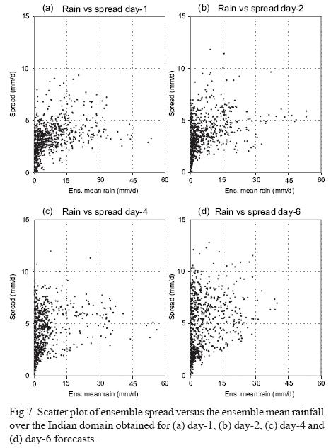
Figure 7 (a–d) shows the scatter plot of ensemble spread versus the ensemble mean rainfall over the Indian domain obtained for day–1, day–2, day–4 and day–6 forecasts. The spread amount is shown as a function of rainfall produced by the model in the figure. As already mentioned, ensemble spread represent the uncertainties in the model predictions. If these spreads are due to uncertainties in the diabatic processes in the model (diabatic processes are generally referred to as the stochastic–dynamic processes), uncertainties shall be large when there is a large amount of rainfall. In the tropical monsoon region, convection dominates the diabatic processes. Therefore, when rainfall is more in the ensemble mean, it is expected that uncertainties in the computations of convective heating/cooling and moistening/drying shall be large. At this stage, the ensemble spread shall be large. With similar argument, it can be said that the ensemble spread shall be less if the rainfall produced by the model is lower. By analyzing the figure, a couple of important conclusions can be made. As seen in Figure 6, and as expected, the ensemble spread increases as the forecast length increases from day–1 to day–6. When the rainfall amount increases (for each day of forecast), the spread is also seen to have increased. However, there is no linearity in the increase of spread with the rainfall amount. After about 20 mm/day of rainfall, the spread does not, by and large, increase beyond about 8 mm/day. One more important aspect seen in this figure is that when the rainfall amount is low, the spread is quite large. When the rainfall amount is between 0–10 mm/day, the spread ranges from 0 to 10 mm/day. Therefore, the forecasts of probability of rain or no rain will have a lot of problems if these forecasts are used without proper calibration. Further, while issuing forecasts for light rain, the uncertainties associated with these forecasts will also be quite large. A relatively large spread for low rainfall amounts could be associated with the tuning of the convective scheme. In the Kuo–type convection scheme, cumulus convection is triggered in the model when the moisture convergence at a grid point exceeds a threshold value and if the layer is convectively unstable. Several sensitivity experiments with the tunable parameters indicate that triggering of convection/rainfall is too frequent in the model.

3.4 Systematic errors

When ensemble forecasting was first implemented at major NWP centers (e.g., Toth and Kalnay, 1993; Molteni et al., 1996) it was designed to assess forecast uncertainty related to errors present in the initial conditions. The initial errors project on atmospheric instabilities and amplify in time, leading to loss of usability of forecasts beyond a period of time. Forecast uncertainty also arises due to simplifications such as parameterized schemes introduced in numerical models. The use of such models leads to the emergence of errors, in addition to those due to inaccurate initial conditions. Part of the overall error due to model imperfectness can be classified as systematic, and another part as random or stochastic. Figure 8 (a, b) shows the difference of day–3 and day–1 forecast rainfall (mm/day) and difference of day–6 and day–1 forecast rainfall (mm/day) over the Indian region. These plots are from the control model run at T80L18 resolution. If the model has no tendency in systematic bias, then the difference of day–3 and day–1 and similarly the difference of rainfall between day–6 and day–1 should be zero. From the figure, it is seen that the model has a systematic tendency to increase rainfall amount in forecasts over India and central Bay of Bengal as the forecast length increases from day–1 to day–6. In Figure 8a, the model has produced more rain in day–3 as compared to day–1 over eastern parts of India which extends to peninsular part. By day–6, this increase in rainfall is further enhanced and it spreads to more part of the central Bay of Bengal. It is worth noting that the ensemble spread also becomes more over the same region where rainfall amount is enhanced as the forecast length increases. Over the equatorial Indian Ocean, the model tends to dry up with about 2–4 mm/day less rainfall in day–3 as compared to day–1 forecasts. However, as the model is run till day–6, the rainfall amount is further reduced over this region and the deficit of rainfall in day–6 is 6–8 mm/day as compared to day–1. This systematic bias is very significant in the sense of interpretation of medium–range forecasts over the Indian region. This systematic error of the low resolution T80L18 model is not the same in the high resolution version (T170L28) of the model (figure not shown). Whereas in the the high resolution model tends to rain more over the eastern parts in first two days of forecast, after that no increase in rainfall is seen in this region. The high resolution model also does not have any systematic tendency to reduce or increase rainfall over the neighboring ocean.

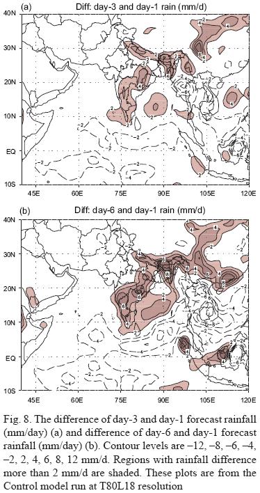
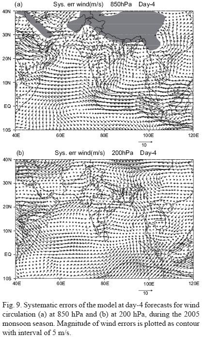
Figure 9a shows the systematic errors of the model at day–4 forecasts for wind circulation at 850 hPa during the 2005 monsoon season. Figure 9b shows the same figure at 200 hPa. These are systematic errors computed using control runs of the T80L18 model. The model has very large easterly bias over the entire equatorial Indian Ocean at 850 hPa. Easterly bias over the Indian Ocean and the Arabian Sea tend to weaken the monsoon circulation over the region by day–4 forecasts. At 200 hPa, the model has a tendency to weaken the subtropical high and weaken the Tibetan anti–cyclone. The tropical easterly jet is also weaker in forecasts. These large systematic errors in wind circulation affect the monsoon circulation over the Indian region rendering the monsoon forecasts less usable.

Earlier, it was noticed that the model has a tendency to increase rainfall over the southern and eastern parts of India as the forecast hours increases. The ensemble spread also increases with forecast length over the same region. The fact that the model has a strong southerly bias over the region and this bias intensifies along the forecast length, suggests that the warm and moist air from the equatorial Indian Ocean is brought by the wind bias to this region and the rainfall over this region is increased further. Therefore, large systematic model errors dominate the forecast patterns as forecast length increases. These results suggest that for getting optimum benefit from the ensemble prediction system, attempts have to be made to reduce the systematic biases in the model as the breeding method only takes care of the uncertainties in the initial conditions and not model–related errors.

The skill of the ensemble prediction system can be seen from the comparison of the errors of forecasted wind field with observations. Figure 10a shows the root mean square error (RMSE) of wind at 850 hPa from ensemble mean and control runs at day–5 forecasts. This comparison is made against all radiosonde observations over India, and is considered to be a very stringent verification metric. Figure 10 (b) shows the same field for 200 hPa. The comparisons are made on day by day basis for entire July month. It is seen that at both the levels, the RMSE values are smaller for the ensemble mean as compared to the control run. The range of improvement by the EPS is about 1 m/s at 850 hPa and about 2 m/s at 200 hPa. There are of course several days in the season, when improvement obtained from the EPS system is higher than that shown in the figure. It may be noted that the large wind errors are caused mostly by the systematic errors of the model, which in turn are due to inadequacies in the model physics. A recent study (not described here) shows that even another state of the art global model at much higher resolution (T254L64) provided almost the same improvement in wind RMSE as the one shown here. Therefore, while changing model resolution, or while implementing ensemble prediction system at lower resolution, a cost benefit analysis should be made. It is worth noting that an EPS system with lower resolution shall allow more number of ensemble members to be run than running a single high resolution expensive global model. If the systematic errors of a low resolution global model are reduced, that model can provide as much better medium–range weather forecasts in an EPS system.

 

4. Conclusions

At NCMRWF, real–time global data assimilation system and global forecast models are run every day for preparing medium–range weather forecasts. Two different global models at T170L28 and T80L18 resolutions are used for the present study. Ensemble forecasting techniques involves generation of multiple forecasts as a function of the uncertainties in the analysis. The goals of ensemble forecasting are to increase the average forecast accuracy, to estimate the likelihood of various events, and to estimate the forecast spread which can be used as an indicator of the forecast skill. For the present study, the breeding method developed by Toth and Kalnay (1993) has been implemented for the generation of the initial perturbations. Four independent breeding cycles using the operational T80L18 global spectral model have been used to generate eight member ensemble initial perturbations. Experimental forecast runs with these 8–member ensembles have been carried out and results are analyzed for a monsoon season.

A comparison of the forecast rainfall generated by the coarse resolution T80L18 global model against the high–resolution T170L28 model shows that the T80L18 model broadly brings out the essential features of the rainfall distribution during the monsoon season under consideration. However, the magnitude of rainfall forecasted by the coarse resolution model is too low compared to observation as well as that of T170L28 model. Spatial distribution of rainfall from the high resolution model agrees well with available observed data. The ensemble mean of rainfall forecasts shows that over the larger domain such as the Gangetic plains, the EPS brings out the monsoon activity (active and weak spells of rainfall) reasonably well six days in advance. However, when the region under consideration is shifted to the eastern parts of India, the ensemble mean rainfall is good only in short–range. The ensemble spread becomes quite large from about day–4 forecast and beyond. A shift in the phase of monsoon activity is seen in rainfall forecasts as compared to observations. After examination of the rainfall pattern from day–1 to day–6 forecasts by the model and the ensemble spread, it appears that in the region, when the rainfall amount increases (for each day of forecast), the spread is also seen to have increased. However, there is no linearity in the increase of spread with the rainfall amount.

The model has a systematic tendency to enhance rainfall activity over the central Bay of Bengal and eastern parts of India as the length of forecast is increased. Further, the amount of rainfall enhancement and regions covered also increases with length of forecast. At the same time, the model tends to dry up over the equatorial Indian Ocean region. In circulation fields too, the model has large systematic errors. Over some parts of the Indian region, the magnitude of this systematic error is enhanced as the forecast length is increased. These results suggest that to obtain maximum benefit from the ensemble prediction system, the systematic biases in the model must be reduced as the breeding method only takes care of the uncertainties in the initial conditions and not of model–related errors. One of the main findings of this study is that the EPS system is able to reduce RMSE of wind errors to some extent over the Indian region.

 

References

Anthes R. A., 1977. A cumulus parameterization scheme utilizing a one– dimensional cloud model, Mon. Wea. Rev. 105, 270–286.         [ Links ]

Basu S., G. R. Iyengar and A. K. Mitra, 2002, Impact of non–local closure scheme in simulation of monsoon system over India, Mon. Wea. Rev. 130, 161–170.         [ Links ]

Bohra A. K., S. Basu, E. N. Rajagopal, G. R. Iyengar, M. Das Gupta, R. Ashrit and B. Athiyaman, 2006. Heavy rainfall episode over Mumbai on 26 July 2005: Assessment of NWP guidance. Curr.Sci. 90, 1188–1194.         [ Links ]

Buizza R., M. Miller and T. N. Palmer, 1999. Stochastic simulation of model uncertainty in the ECMWF ensemble prediction system. Q. J. R. Meteorol. Soc. 125, 2887–2908.         [ Links ]

Harshvardhan R. D., D. A. Randall and T. G. Corsetti, 1987. A fast radiation parameterization for general circulation models, J. Geophys. Res. 92, 1009–1016.         [ Links ]

Hong S.–Y. and H.–L. Pan, 1996. Nonlocal boundary layer vertical diffusion in a medium–range forecast model. Mon. Wea. Rev. 124, 2322–2339.         [ Links ]

Houtekamer P. L., L. Lefaivre, J. Derome, H. Ritchie, and H. L. Mitchell, 1996. A system simulation approach to ensemble prediction. Mon. Wea. Rev. 124, 1225–1242.         [ Links ]

Houtekamer P. L. and L. Lefaivre, 1997. Using ensemble forecasts for model validation. Mon. Wea. Rev. 125,2416–2426.         [ Links ]

Kanamitsu M., 1989. Description of the NMC global data assimilation and forecast system. Weather Forecast. 4, 335–342.         [ Links ]

Kanamitsu M., J. C. Alpert, K. A. Campana, P. M. Caplan, D. G. Deaven, M. Iredell, B. Katz, H.–L. Pan, J. Sela and G. H. White, 1991. Recent changes implemented into the global forecast system at NMC. Weather Forecast. 6,425–435.         [ Links ]

Kar S. C., 2002. Description of a high–resolution global model (T170/L28) developed atNCMRWF. Research Report 1/2002, NCMRWF, 28 pp.         [ Links ]

Kar S. C., G R. Iyengar, S. Das, S. Basu, J. P. George and A. K. Mitra, 2002. Improvements in the NCMRWF global atmospheric modeling system. In: Weather and Climate Modeling (S. V. Singh, S. Basu and T. N. Krishnamurti, Eds.). New Age International Publishers, 1.15–1.23.         [ Links ]

Kar S. C., K. Rupa, M. Das Gupta and S. V. Singh, 2003. Analyses of Orissa super cyclone using TRMM (TMI), DMSP (SSM/I) and oceanSat–I (MSMR) derived data, Global Ocean Atmos. Sys. 9, 1–18.         [ Links ]

Kobayashi C., K. Yoshimatsu, S. Maeda and K. Takano, 1996. Dynamical one–month forecasting at JMA. Preprints of the 11th AMS Conference on Numerical Weather Prediction. Aug. 19–23, Norfolk, Virginia, 13–14.         [ Links ]

Kuo Y. H., 1974. Further studies of the parameterization of the influence of cumulus convection of large–scale flow. J. Atmos. Sci. 31, 1232–1240.         [ Links ]

Mani N. J.,E. Suhas and B.N. Goswami,2009. Can global warming make Indian monsoon weather less predictable. Geophys. Res. Lett. 36, L08811, doi:10.1029/2009GL037989.         [ Links ]

Molteni F., R. Buizza, T. N. Palmer and T. Petroliagis, 1996. The ECMWF ensemble system: Methodology and validation. Q. J. R. Meteorol. Soc. 122, 73–119.         [ Links ]

Pan H–L. and L. Mahrt, 1987. Interaction between soil hydrology and boundary layer developments. Bound.–Lay. Meteorol. 38, 185–202.         [ Links ]

Parrish D. F. and J. C. Derber, 1992. The National Meteorological Centre's spectral statistical interpolation analysis system. Mon. Wea. Rev. 120, 1747–1763.         [ Links ]

Rajeevan M., J. Bhate, J. D. Kale and B. Lal, 2006. High resolution gridded rainfall data for the Indian Region: Analysis of break and active monsoon spells. Curr. Sci. 91, 296–306.         [ Links ]

Rathore L. S. and P. Maini, 2008. Economic impact assessment of agro–meteorological services of NCMRWF, Report No. NMRF/PR/1/2008, published by NCMRWF, India, 104 pp.         [ Links ]

Richardson D. S., 2000. Skill and economic value of the ECMWF ensemble prediction system, Q. J. R. Meteorol. Soc. 126, 649–668.         [ Links ]

Tiedtke M., 1983. The sensitivity of the time–mean large–scale flow to cumulus convection in the ECMWF model. ECMWF Workshop on Convection in Large–Scale Models, 28 November. Reading, England, 297–316.         [ Links ]

Toth Z. and E. Kalnay, 1993. Ensemble forecasting at the NMC: The generation of perturbations. Bull. Amer. Meteorol. Soc. 74, 2317–2330.         [ Links ]

Toth Z. and E. Kalnay, 1997. Ensemble forecasting at NCEP and the breeding method. Mon. Wea. Rev. 125,3297–3319.         [ Links ]

Zhu Y., Z. Toth, R. Wobus, D. Richardson and K. Mylne, 2002. On the economic value of ensemble based weather forecasts. Bull. American Meteorol. Soc. 83, 73–83.         [ Links ]