


Serviços Personalizados
Journal
Artigo
 texto em
  Inglês (pdf)
 Artigo em XML
 Referências do artigo
 Enviar este artigo por email
Indicadores
-
 Citado por SciELO
 -
 Acessos
Links relacionados
-
 Similares em
SciELO
Similares em
SciELO
Compartilhar

 Permalink
Agrociencia
versão On-line ISSN 2521-9766versão impressa ISSN 1405-3195
Agrociencia vol.50 no.6 Texcoco Ago./Set. 2016
Natural Renewable Resources
Prediction of land use change/forest cover in Mexico Trough transition probabilities
1Centro de Investigación y Docencia Económicas, División de Economía. Carretera MéxicoToluca No. 3655. Colonia Lomas de Santa Fe, México D.F. México. 01210. (juanmanuel.torres@cide.edu).
2Instituto Nacional de Investigaciones Forestales, Agrícolas y Pecuarias. México. (magana.octavio@inifap.gob.mx), (moreno.francisco@inifap.gob.mx).
This article presents a prediction model for land use change/ forest cover through the projection of transition probability matrices. The prediction model uses the information of forest cover/land use generated by INEGI in 1993 and 2000, and uses the information from 2007 to validate the model. The covers at national scale (1:250,000) are broken off by state and a transition probability matrix was generated of the types of vegetation/land use for each state. Then, through a system of equations of logit models, the transition probabilities were related to climate, physical and socioeconomic variables, in order to explain the change dynamics of forests and rainforests in the country. This methodology allows analyzing the changes in each type of vegetation isolated from the different uses, with which the prediction and understanding of the change dynamics of land cover are improved. This allows clearly identifying the causes of deforestation and provides information to develop and focus better policy instruments linked to the reduction of deforestation. The results showed that the basic transitions of forest regions to crops and grasslands follow different dynamics in forest and in rainforests. It is noteworthy that when identifying differences in the transitions, conditions can be distinguished where land use change can be persistent and where it is not.
Keywords: Land use change/cover; deforestation; transition matrices; logit models
Este artículo presenta un modelo de predicción del cambio de uso/cobertura del suelo a través de la proyección de matrices de probabilidades de transición. El modelo de predicción usa la información de cubierta forestal/uso del suelo generada por el INEGI en 1993 y 2000 y utiliza la información de 2007 para validar el modelo. Las coberturas en escala nacional (1:250,000) se cortaron por estado y se generó una matriz de probabilidades de transición de tipos de vegetación/uso del suelo por cada estado. Después, a través de sistemas de ecuaciones de modelos tipo logit, se relacionaron las probabilidades de transición con variables climáticas, físicas y socioeconómicas para explicar la dinámica de cambios de los bosques y las selvas del país. La metodología generada permite analizar los cambios de cada tipo de vegetación aislada en los usos diferentes, con lo que se mejora la predicción y el entendimiento de la dinámica de cambio de la cobertura del suelo. Esto permite identificar claramente los causales de deforestación y brinda información para desarrollar y focalizar mejores instrumentos de política pública vinculados con la reducción de la deforestación. Los resultados mostraron que las transiciones básicas de regiones arboladas a cultivos y pastizales siguen dinámicas diferentes en bosques que en selvas. Resulta notable que al identificar diferencias en las transiciones se pueden diferenciar condiciones en las que el cambio de uso puede ser persistente y en las que no lo es.
Palabras clave: Cambio de uso/cobertura del suelo; deforestación; matrices de transición; modelos tipo logit
Introduction
The loss of plant coverage brings with it the degradation of the genetic reserve, the loss of potential for use of the multiple environmental goods and services provided by ecosystems for human and biological wellbeing, as well as global warming, alteration of water and biogeochemical cycles, introduction of exotic species, extinction of native species, and loss of habitat (Cairns et al., 2000; Velázquez et al., 2002).
The global deforestation process reached alarming levels by the 1980s (Chomitz and Gray, 1996), although between 2000 and 2010 this process showed signs of significant reduction. Nevertheless, several countries, mostly in Africa, Latin America and Southeast Asia, maintain high levels of deforestation, particularly in their tropical forests (FAO, 2012; Hosonuma et al., 2012). Despite the reduction of deforestation, the figures are still high, and FAO (2012) points out that in the 1990s around 16 million ha of forests in the world disappeared, compared to the 13 million ha lost in the prior decade.
In México, there are efforts both to carry out the cartography of land use (INEGI, 2000, 2007; 2012; SARH, 1992; 1994; Dirzo and Masera, 1996), and to evaluate the space-time dynamics of plant coverage (Velázquez et al., 2002; López, 2012; Rosete et al., 2014), an analysis known as land use change/land cover (Berry et al., 1996). Many of these analyses were carried out with diverse objectives, criteria (cover evaluation and classification) and scales (from 1:50 000 to 1:8 000 000), so that the analyses of land cover /land use change are not homogeneous, and the results are not comparable in most cases (Velázquez et al., 2002).
The analysis of the dynamics of land use change in México has been performed in various manners: 1) comparative spatial analyses that identify the change patterns with several scales (Mendoza and Dirzo, 1999; Velázquez et al., 2002; 2003); 2) analyses that identify a causal relation between institutional variables (Bray et al., 2004; 2008 ), socioeconomic and physical ones, with the use of dynamic or static models at State (Torres and Flores, 2001), municipal (Deininger and Minten, 2002), local or regional (Dirzo and García 1992; Mendoza and Dirzo, 1999; Ochoa and González, 2000; Trejo and Dirzo, 2000; Chowdhury, 2006; Castillo-Santiago et al., 2007) community (Alix-García et al., 2005; Alix-García, 2007; López, 2012), or even at pixel level (Muñoz et al., 2003). They all have methodological advantages and disadvantages given the territorial level used and the information available.
This study presents a methodology to predict the changes of land use/cover with forestry use, and two objectives: the predictive one, per se, and that of identifying and ordering possible causes of this dynamic. The study differs from others performed with the same State scale because it disaggregates the process of land use change/cover in the different resulting covers, so that the response variable is not the total change in use, but rather an approximation to the surface converted from forest/rainforest to a different use/cover. With this disaggregation, the hypothesis is set out that processes of land use change/cover vary according to the type of vegetation (forest or rainforest) and the resulting use/cover.
Materials and methods
Model
A transition matrix (TM) of land use/cover was integrated when evaluating the different covers in two successive periods of time (Table 1), and compares the land use/cover maps for 2000 and 2007 in México with their respective annual change rates. Once the TM was integrated, the transition probability matrix (TPM) is calculated; that is, the matrix that shows in each one of its entries the probability (p ij ) for a formation to change from status i to j in the following evaluation period. For example, according to the information in Table 1, the probability for the forest cover in the year 2000 to change into induced grassland in the next period (2007) is 37/34,163=0.00109. The change probabilities (p ij ) must satisfy the restriction that their sum from formation i must be equivalent to the unit, that is:
Table 1 Plant cover transition matrix (ha x 1,000) between years 2000 and 2007.
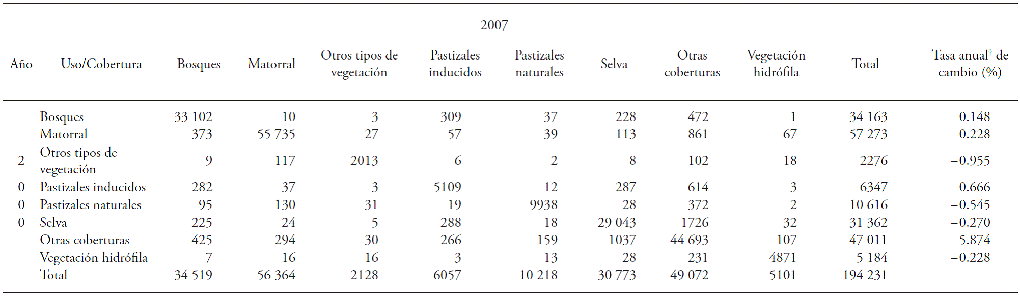
†Rate (d) calculated as [(S 2/S 1)(1/n)]-1; where n represents the number of years between the cover in period 1(S 1) and period 2 (S 2). The Table was elaborated based on Series II and III from INEGI.
Assuming homogeneity in the events that cause the transition, the TPM follows a first order Markovian process (Balzter, 2000), so that the change probability of the land use/cover depends only on the current condition; from this, the history of the events does not have any relation with the future transition probabilities; therefore, it is implicitly assumed that the set of causes of the transition is the same throughout time. Under this assumption, it is possible to predict a future state by just knowing the current state, and the TPM through the following equation:
where bt is the column vector that represents the fraction of land in each one of the m categories in the period and P is the TPM of size m x m. For example, the distribution of use/ cover for period t+3 would be given by: b
t+3
= Pb
t+2
= P
2
b
t+1
= P
3
b
t
; in fact it is possible to identify a stationary status, that is, the transition probability after n periods (p
j
), when
The transition probabilities (p ij ) can be assumed to be constant (Balzter, 2000), or variable, according to a set of drivers (Chomitz and Gray, 1996; Sandoval and Real, 2005), with which certain adaptability is incorporated into the process. The contribution of these causes is modelled by the Markov chain modified equation to the form: b t-1 =P[f(t)] bt; where f(t) is a function that defines p ij in time t based on a set of variables through a general model. This last procedure is the one used in this study to integrate the effect of socioeconomic, physical and climate variables in the definition of land use. This methodology was used successfully to evaluate the effect of temperature and density on mite populations (Woolhouse and Harmsen, 1987), and in plant cover models, which include socioeconomic variables or climate conditions, and even indicators of the composition of the types of covers (Henderson and Wilkins, 1975; Marsden, 1983; Ludeke et al., 1990; Chomitz and Gray, 1996; Balzter, 2000; Benabdellah et al., 2003; Sandoval and Real, 2005).
With the objective of enhancing the information to adjust the model, each State in the federation was considered as an independent unit. For this purpose, the covers at the national scale (1:250 000) were broken off by State and a TPM of the types of land use/cover was generated for each State. The transition probabilities (p ij ) were modelled by a set of variables through a logistic model of the form:
where b represent parameters of the model and the x correspond to each one of the explicative variables of the variation in the transition probability. From construction, the pij have the restriction of
there ln(pij/(1-p ij )) is the logit (lgtij) from p ij , band x have the same notation as before, whereas the a represent parameters of the model associated to the endogenous variables (y) within the system. These variables represent variables related bi-directionally within each equation of the model, as for example the same transition probability of other formations or, in an extensive case, the same socioeconomic or accessibility conditions. The p ij can depend on other transition probabilities within the same system, with which the errors from each equation in the model can be correlated. Therefore, the adjustment was performed with the procedure model (PROC MODEL) from SAS®, using the adjustment variant with maximum likelihood estimators of complete information.
Based on the adjusted models and the information for year 2000, the predicted transition probabilities (p ij ) were calculated for each use/cover and in each State, from which the state TM was recovered for the following period (2007). Then, with the sum of the State TMs, a national TM with its respective TPM was integrated. The latter was compared statistically with the TPM calculated from Series IV (INEGI, 2012), through a x2 test. It must be clarified that the projection and measurement periods could be partially equivalent, given that Series II was published in the year 2000, but it was elaborated from 1994 to 1999, whereas Series III was elaborated from 2003 to 2005, and published in 2007. Therefore, the interval of projection assumed between Series II and Series III is 7 years, and from 1995 to 2002, the same that are assumed for the measurement interval between Series III and IV (INEGI, 2012).
Data
The cartographic information used to estimate the transition matrices was Series II (INEGI, 2000) and Series III (INEGI, 2007). The breakoff of State covers was carried out based on the State cover published by INEGI (INEGI, 2000a). Given that the nomenclature of covers integrates a high number of categories, they are regrouped into categories (Table 2).
Table 2 Description of categories used to standardize nomenclature of covers from different formations, based on the nomenclature by INEGI (Victoria et al., 2011).
| Categoría de tipo de vegetación | Abreviatura | Descripción de la categoría |
|---|---|---|
| Bosque | b | Todos los bosques de clima templado, incluyendo matorral de coníferas |
| Matorral | m | Todos los tipo de matorral, chaparral y mezquital incluyendo vegetación de desiertos arenosos |
| Otras coberturas | oc | Zonas urbanas, cuerpos de agua y cultivos |
| Otros tipos de vegetación | otv | Pastizal gipsófilo y halófilo, vegetación de dunas y palmar |
| Pastizal natural | pn | Cualquier pastizal natural incluyendo sabanas, pastizal-huizachal y pradera de alta montaña |
| Pastizal inducido y cultivado | pi | Pastizales inducidos y cultivados |
| Selva | s | Todos los tipos de selva |
| Vegetación hidrófila | vh | Manglar, tular, popal y vegetación de galería |
The set of explicative variables of changes in transition probabilities was selected according to availability, aligning with the projection date (information up to year 2000; Table 3), and recommendations by Balzter (2000), Benabdellah et al. (2003), and Sandoval and Real (2005).
Table 3 Sources of information of variables used in the prediction models.
| Variable | Fuente de información |
|---|---|
| Desviación estandar. Número de incendios forestales por año | CONAFOR (2005) |
| Consumo de leña combustible (m3 per cápita) | Díaz y Masera (2003) |
| Temperatura máxima (°C) | CONABIO (2001) |
| Precipitación anual (mm) | CONABIO (2001) |
| Educación (Proporción de población > 18 años alfabeta) | INEGI (2000b) |
| PIB per cápita año 2000 (Miles $/año) | INEGI (2000c; 2000d) |
| PIB municipal (Miles $/año) | INEGI (2000c) |
| Densidad caminos (km/km2) | IMT (1999) |
| Migración neta (Miles personas) | CONAPO (2000) |
| Proporción de la superficie en cultivo agrícola | SAGARPA (2004) |
| Proporción de la población rural | INEGI (2000b) |
| Proporción de la superficie en ejidos y comunidades | INEGI (2000a; 2004) |
| Densidad de la población rural | INEGI (2000b) |
Results and discussion
Transition from forest to other formations
The predictions of transition from forest to forest (f-f), forest to shrub (f-s), and forest to other covers, among which are considered crops and urban zones (f-oc), showed satisfactory adjustments judging from the statistics for goodness of fit of the system of equations, although the transition from forest to induced grasslands (f-ig) did not. The transition from forest to natural grassland (f-ng) had low frequency, so it was considered as a false change (Table 4).
Table 4 Estimations of the model of simultaneous equations of transitions from forest to other formations. The response variable is the logit of the referred transition probability.
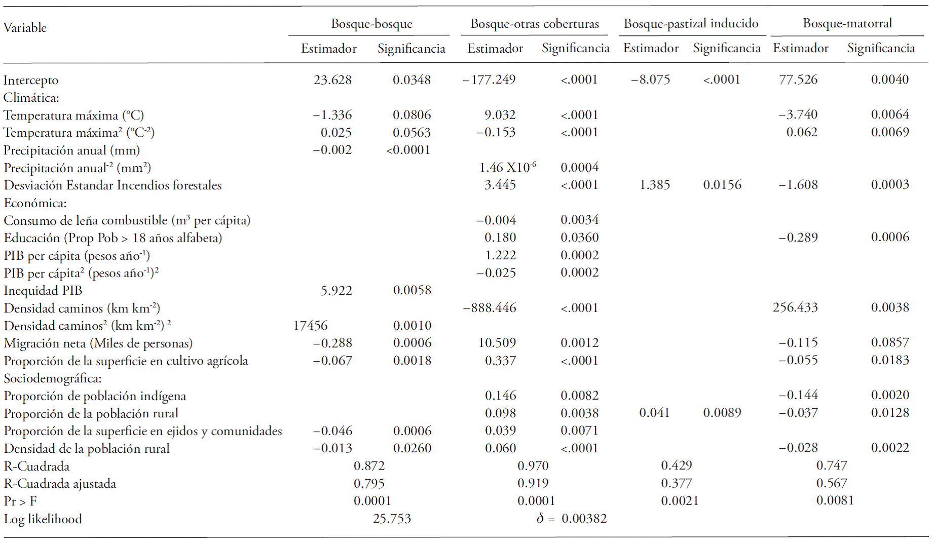
The prediction of the most important transition, f-f, which measures the permanence of this cover, showed that an increase in precipitation reduces the probability of transition, that is, promotes the change from forest to other uses. The effect of temperature is: with higher maximum temperature, a lower permanence of the forest area is verified; however, the behavior is reversed when the maximum temperatures are above 26 °C. The behavior of these two variables is closely linked to the most frequent change in use of this coverage, which is directed towards agricultural crops and urban zones where lands with good precipitation and maximum temperatures that are not extreme are demanded. Therefore, in the forest localities with higher temperature and lower humidity, there will be greater conservation of the forest land, which is linked to its lower agricultural aptitude.
The Gini coefficient of the GDP distribution among municipalities was taken as proxy of the presence of poles of wealth in the State. The variable is related directly to the forest’s probability of permanence, which can be interpreted as the effect of the poles of wealth to attract population, which finally translates into lower human pressure on the forest. The accessibility, measured through the road density (km km-2), is also related to the possibility of having infrastructure to perform other productive activities that take pressure away from the forest. The variable could be considered endogenous (i.e. the forest’s permanence can attract its exploitation and foster the construction of roads), but the form of the response variable avoids this problem.
Net migration was also highly significant to describe the process of forest conservation; the presence of a higher number of individuals who were not born in the geographic unit promotes the change from forest use to other uses. The variable can be related to two effects: that of a higher population pressure and the one related to customs in land use, although the first has been captured with the variable “density of rural population”.
The proportion of agricultural surface was significant and with an inverse relation. This variable is related to technological availability and markets associated to the agricultural activity that promote the expansion of the agricultural frontier. Also, the proportion of surface in ejidos and communities was significant and with an inverse relationship. This proportion does not represent ejidos/communities with forest, so it is not related to the higher or lower conservation that can be carried out in forest communities. In sum, all the variables used to explain the permanence of the forest were significant and with the expected sign.
The transition forest to other covers (f-oc), basically crops and urban development, is the most important because of its frequency. Albeit it is related to climate variables, its most important cause is economic variables. The climate variables show that maximum temperatures above 29.5 °C are not apt for crops, which is why the change from forest use is less attractive. The humidity also influences the availability of the terrain for agricultural use, which is why when there is higher precipitation, the probability for transition is higher. The change from forest use is also related to the standard deviation of forest disasters; with higher variation in the number of these events, there is higher probability of change from forest use, which suggests that large clearings, resulting from disasters, could be taken advantage of to open cultivation lands.
Within the economic variables, there is the per cápita GDP and accessibility. The first shows that when there is greater wealth there is higher change of forest land use up to a threshold (approximately $24 000 per year), from which the probability of use change is reduced, which is a similar effect to the trend of Kuznets environmental degradation (Stern et al., 1996). The coefficient associated to the road density shows that higher accessibility is not necessarily related to a loss of temperate forests, as is thought that it happens in tropical forests (Chomitz, 2007), and in this case, the model suggests that a higher accessibility reduces the pressure on the forest, presumably through the development of other economic activities and their effect on migration and the development of economic attraction poles.
In a manner analogous to the effect on f-f conservation, the net migration and the surface of agricultural crops increase the probability of transition f-oc. The variables density of rural population, proportion of rural population, and proportion of surface in ejidos and communities have an inverse behavior to the one discussed for the conservation of the forest (f-f ). In this group of sociodemographic variables, it stands out that the proportion of indigenous population increases the transition from forest to crops or urban development. The variable is not linked to the indigenous population that inhabits the forest, so its interpretation should be done with reserve.
The transition f-ig is the second most important one because of its magnitude, although it is quite limited to the States of Chiapas, Jalisco, Oaxaca and Estado de México. The transition is closely related to extreme events (fires) that apparently create large clearings, which are induced into forming grasslands, reason why it seems likely that some of these events are of anthropogenic origin, with this intention. Another variable directly related to this transition is the proportion of rural population, variable that shows that this transition is highly dependent of human pressure on the forest.
The transition f-s is not very common and its presence is higher in the States of Baja California, Coahuila, Guerrero and Querétaro. Among the important economic variables that define this transition, the ones that stand out are education (with inverse relation), road density (direct relation), net migration (inverse relation), and the proportion of surface with agricultural use. The higher road density promotes the transition surely as a result of the effect of the ill-handled change of land use. The model also shows that insofar as there is less arable surface, the transition f-s is more likely. These relationships strengthen the hypothesis that the transition f-s is linked to the abandonment of marginal cultivation lands that were originally forest (Chomitz, 2007).
Transition from rainforest to other formations
The results of the adjustment of the system of equations related to the transition from rainforest to other formations showed that the prediction of transition from rainforest to crop (rf-oc), rainforest to induced grassland (rf-ig), and the permanence of rainforest (rf-rf) adjusted satisfactorily, and the adjustments were superior to those of the false transition rainforest to forest (rf-f) (Table 5).
Table 5 Estimations of the model of simultaneous equations of the transitions from rainforest to other formations. The response variable is the logit of the transition probability referred.
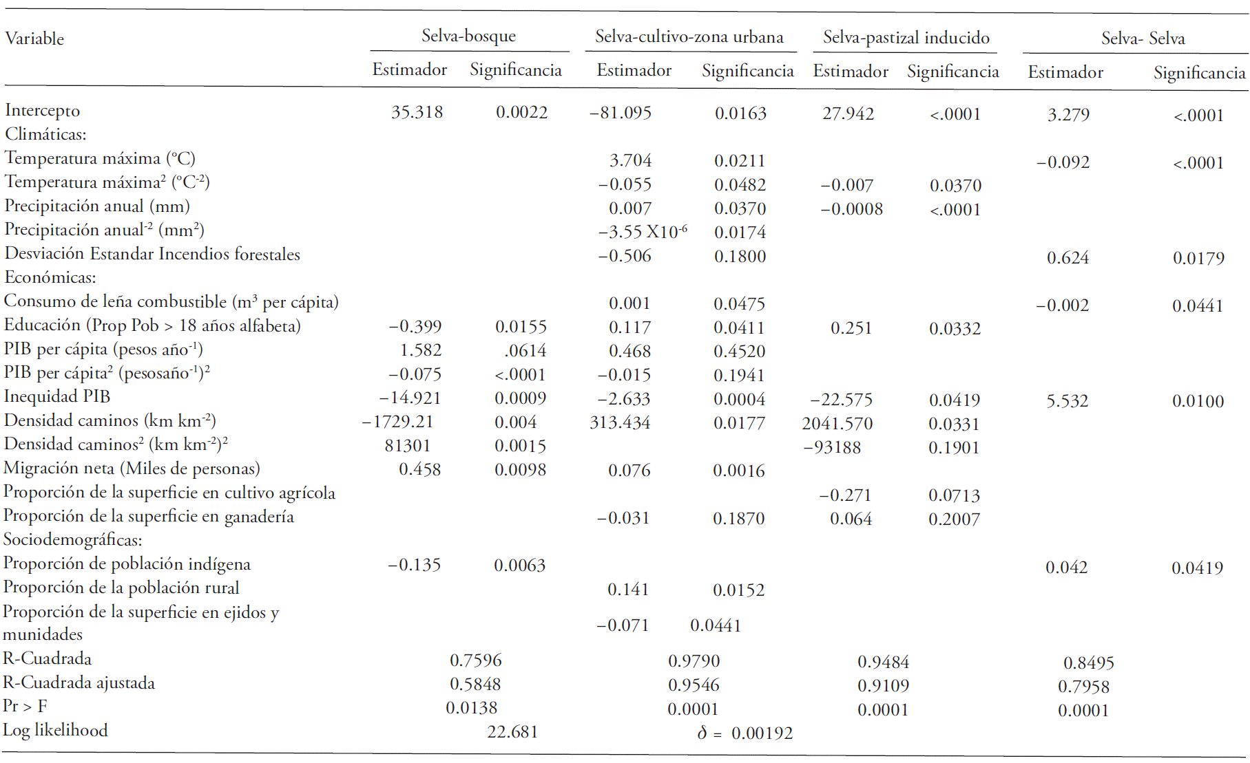
The variation in the number of forest fires, the presence of economic poles, the presence of indigenous population and the consumption of firewood were the variables with greatest weight in the conservation of the rainforest (rf-rf). The temperature has less significance but is consistent with the result obtained for the transition rainforestcrop/urban zone and aligned with the presence of variations in the number of fires.
Consumption of firewood is a variable that is inversely related to the probability of the rainforest permanence. This relation evidences not only the degradation of the rainforest as a result of the extraction of firewood, but also the change of use with traditional cultivation systems (slash and burn) applied massively. The variable proportion of rural population was significant and had a positive effect, which is linked to the prior discussion. Among the economic variables, it was confirmed that inequity in the GDP, promoted by important economic centers, attracts workforce and decreases pressure on the change of rainforest use.
The transition rainforest-crop/urban zone (rfoc) depends on the temperature, the variation in disasters, and the precipitation. Results show that the transition increases in localities with higher precipitation up to the maximum limit of 1 050 mm, value from which the probability of transition is reduced. This interval is clearly related with the interval where agricultural productivity is higher; outside this interval, the desirability for land use change is reduced. The adjustment shows that when there is higher wealth, the probability of transition in a quadratic relation that resembles the Kuznets’ (Stern et al., 1996) curve of environmental degradation is higher. Road density is another relevant variable that shows a direct relationship with the change in rainforest land use, in contrast with the behavior observed in temperate forests and in accordance with the one observed in other regions of the world for tropical forest (Chomitz, 2007).
Other important economic variables to define the transition rainforest-crop/urban zone (rf-oc) are firewood consumption (discussed above); level of education, with a direct relation; and inequity in per cápita GDP distribution, with an inverse relation, which was discussed in prior paragraphs. Again, the variable net migration stands out with a positive relation, indicating that when there is greater presence of individuals who are not native to the zone, there is a higher impact on land use change. Another relevant variable is the proportion of the surface used for livestock production, which has an inverse relation with the transition from rainforest to crop and thus shows some substitution in land use. The contrary case occurs with the transition to induced grassland, where there is complementarity.
The higher proportion of rural population has a direct effect, which suggests the strong effect of population density on rainforest conservation. In this sense, it is observed that if the higher density is concentrated in ejidos or communities, then the effect of use change is reduced, presumably because this type of trend shows lower possibility of investment in the livestock production sector.
The transition rf-ig is reduced both with the increase in temperature and in precipitation. These variables impact directly on the reduction of livestock productivity. Other economic variables that are related to this transition are education (positive relation), inequity in per cápita GDP distribution (negative relation), road density (positive relation); all of them discussed in prior paragraphs. In this relation, it stands out that the behavior of the variable road density is quadratic, possibly because livestock production development is a secondary stage in land use when the states have greater infrastructure and better economic development. The proportion of agricultural use is an inversely related variable, which confirms a relationship of substitution between the agricultural and livestock use in the rainforest lands cleared.
The transition rainforest-forest, which is assumed to be a false relation, was considered within the system of equations because it has a high frequency and because the rainforests that are highly degraded in drier climates can originate transition formations. Nevertheless, the adjustment is the least satisfactory.
Validation of the model
The model includes the projection of all uses/ covers, but in this article, only the forest and rainforest covers are presented, as well as their transition to covers shown in Table 2. For these covers, a x2 test was performed on the estimated p ij and the p ij obtained from Series IV (INEGI, 2012). For the case of forests, the value of x2=0.0075 (a30.999) was obtained and for the case of rainforests, x2=0.0083 (a30.999). In both cases, there is no evidence to reject the hypothesis that the transition probabilities predicted are not different from those observed, so it is valid to point out that the prediction model through transition probability matrices results in predictions that are statistically similar to the values observed.
Conclusions
The projection procedure generated through transition probabilities, modelled from a set of physical and socioeconomic variables, allows explaining some differences between the dynamics of land use change from forests and rainforests in the country. The procedure enriches the analysis of causes for land use change, and improves the prediction because it incorporates simultaneously the changes from one use/cover to diverse uses, which seem to have different dynamics.
The differences between the causes for land use change per type of forest allow identifying whether the land use change is persistent or only temporal due to the cause and the use at the end of the projection period. Besides, this identification of causes gives information regarding the effectiveness that different public policy instruments could have, which may be applied to reduce deforestation in temperate or tropical forests.
The comparative analysis between the transition matrices predicted and observed showed that the procedure is highly reliable given that the projection was statistically similar to that observed after a period, which could be interpreted as the existence of certain invariability in the causes for land use/cover change.
Literatura citada
Alix-García, J. 2007. A spatial analysis of common property deforestation. J. Environ. Econ. Manage. 53: 141-157. [ Links ]
Alix-García, J., A. de Janvry, and E. Sadoulet. 2005. A tale of two communities: Explaining deforestation in Mexico. World Dev. 33: 219-235. [ Links ]
Balzter, H. 2000. Markov chain models for vegetation dynamics. Ecol. Model. 126: 139-154. [ Links ]
Benabdellah B., K. F. Albrecht, V. L. Pomaz, E. A. Denisenko, and D. O. Logofet. 2003. Markov chain models for forest successions in the Erzgebirge, Germany. Ecol. Model. 159: 145-160. [ Links ]
Berry, M. W., R. O. Flamm, B. C. Hazen, and R. L. MacIntyre. 1996. The land-use change and analysis system (LUCAS) for evaluating landscape management decisions. IEEE Comput. Sci. Eng. 3: 24-35. [ Links ]
Bray, D. B., E. Duran, V. H. Ramos, J. F. Mas, A. Velázquez, R. B. McNab, D. Barry, and J. Radachowsky. 2008. Tropical deforestation, community forests, and protected areas in the Maya Forest. Ecol. Soc. 13: 56. [ Links ]
Bray, D. B. , E. A. Ellis, N. Armijo-Canto and C.T. Beck. 2004. The institutional drivers of sustainable landscapes: a case study of the ‘Mayan Zone’ in Quintana Roo, Mexico. Land Use Pol. 21: 333-346. [ Links ]
Cairns M. A., P. K. Haggerty, R. Alvarez, B. H. J. de Jong and I. Olmsted. 2000. Tropical Mexico’s recent land-use change: a region’s contribution to the global carbon cycle. Ecol. App. 10: 1426-1441. [ Links ]
Castillo-Santiago, M. A., A. Hellier, R. Tipper and B. H. J. de Jong. 2007. Carbon emissions from land-use change: An analysis of causal factors in Chiapas, Mexico. Mitig. Adap.t Strat. Glob. Change 12: 1213-1235. [ Links ]
Chomitz, K. M. 2007. At loggerheads? Agricultural expansion, poverty reduction and environment in tropical forests. World Bank Policy Research Report. Washington, D.C. 284 p. [ Links ]
Chomitz, K. M and D. A. Gray 1996. Roads, Land Use, and Deforestation: A Spatial Model Applied to Belize. World Bank Econ. Rev. 10: 487-512. [ Links ]
Chowdhury, R. R. 2006. Driving forces of tropical deforestation: The role of remote sensing and spatial models. Singapore J. Trop. Geog. 27: 82-101. [ Links ]
CONAFOR (Comisión Nacional Forestal). 2005. Estadística Anual de Incendios Forestales 1970-2004. Coordinación General de Conservación y Restauración Forestal. Gerencia Nacional de Incendios Forestales. [ Links ]
CONABIO (Comisión Nacional para el Conocimiento y Uso de la Biodiversidad). 2001. Catálogo de metadatos geográficos. http://www.conabio.gob.mx/informacion/metadata/gis/rhpri4mgw.xml?_httpcache=yes&_xsl=/db/metadata/xsl/fgdc_html.xsl&_indent=no . (Consulta: Noviembre 2014). [ Links ]
CONAPO (Consejo Nacional de Población). 2000. Índices de marginación 2000. CONAPO, México. 52 p. [ Links ]
Deininger, K., and B. Minten . 2002. Determinants of deforestation and the economics of protection: an application to Mexico. Am. J. Agr. Econ. 84: 943-960. [ Links ]
Díaz, R., y O. Masera (2003). Uso de la leña en México: situación actual, retos y oportunidades. Balance Nacional de Energía. Secretaría de Energía, México DF. pp: 99-109. [ Links ]
Dirzo, R., and M. C. García 1992. Rates of deforestation in Los Tuxtlas, a neotropical area in Southeast Mexico. Cons. Biol. 6:84-90. [ Links ]
Dirzo, R. , y O. Masera. 1996. Clasificación y dinámica de la vegetación en México. In: Criterios y terminología para analizar la deforestación en México. SEMARNAP. México. [ Links ]
Food and Agriculture Organization (FAO) 2012. Global Forest Resources Assessment 2010 Main Report. FAO Forestry paper 163. 340 p. [ Links ]
Henderson, W. and C. W. Wilkins. 1975. The interaction of bush fires and vegetation. Search 6:130-133. [ Links ]
Hosonuma, N., M. Herold, V. de Sy, R.S. de Fries, M. Brockhaus, L. Verchot, A. Angelsen, and E. Romijn. 2012. An assessment of deforestation and forest degradation drivers in developing countries. Env. Res. Lett. 7: 044009. [ Links ]
IMT (Instituto Mexicano del Transporte). 1999. Sistema de Información Geoestadística para el transporte (SIGET), Querétaro, México [cd-rom]. [ Links ]
INEGI (Instituto Nacional de Estadística, Geografía e Informática). 2000. Serie II de uso del suelo y vegetación a escala 1:250 000, México [cd-rom]. [ Links ]
INEGI (Instituto Nacional de Estadística, Geografía e Informática). 2000a. Marco Geoestadístico 2000. Información vectorial. [ Links ]
INEGI (Instituto Nacional de Estadística, Geografía e Informática). 2000b. Censo General de Población y Vivienda 2000. Resultados Preliminares. [ Links ]
INEGI (Instituto Nacional de Estadística, Geografía e Informática). 2000c. Sistema de Cuentas Nacionales de México (SCN). Banco de Información Económica. [ Links ]
INEGI (Instituto Nacional de Estadística, Geografía e Informática). 2000d. XII Censo General de Población y Vivienda 2000, INEGI, 2000 [ Links ]
INEGI (Instituto Nacional de Estadística, Geografía e Informática). 2004. V Censo Ejidal 2001. [ Links ]
INEGI (Instituto Nacional de Estadística, Geografía e Informática). 2007. Conjunto Nacional de Uso del Suelo y Vegetación a escala 1:250 000. Serie III. DGG-INEGI. México. [ Links ]
INEGI (Instituto Nacional de Estadística, Geografía e Informática). 2012. Conjunto Nacional de Uso del Suelo y Vegetación a escala 1:250 000 . Serie IV. DGG-INEGI. México [ Links ]
López F., A. 2012. Deforestación en México: Un análisis preliminar. CIDE, Documento de trabajo 527, 32 p. [ Links ]
Ludeke, A. K., R. C. Maggio, and L. M. Reid. 1990. An analysis of anthropogenic deforestation using logistic regression and GIS. J. Env. Manage. 32:247-259. [ Links ]
Marsden, M. A. 1983. Modeling the effect of wildfire frequency on forest structure and succession in the northern Rocky Mountains. J. Env. Manage. 16: 45-62. [ Links ]
Mendoza, E., and R. Dirzo. 1999. Deforestation in Lacandonia (southeast Mexico): evidence for the declaration of the northern most tropical hot-spot. Biod. Cons. 8:1621-1641. [ Links ]
Muñoz, P. C., G. Alarcón, and J. C. Fernández. 2003. Pixel Patterns of Deforestation in Mexico: 1993-2000. Instituto Nacional de Ecología, SEMARNAT, México. 48 p. [ Links ]
Ochoa G., S. and M. González E. 2000. Land use and deforestation in the highlands of Chiapas, Mexico. App. Geog. 20: 17-42. [ Links ]
Rosete, V. F. A., Pérez D., J. L., Villalobos D., M., Navarro S., E. N., E. Salinas Ch, E.., y R. Remond N. 2014. El avance de la deforestación en México 1976-2007. Madera y Bosques 20: 21-35. [ Links ]
Sandoval, V. y P. Real. 2005. Modelamiento y prognosis estadística y cartográfica del cambio en el uso de la tierra. Bosques 26: 55-63. [ Links ]
SARH (Secretaría de Agricultura y Recursos Hidráulicos). 1992. Inventario Forestal Nacional de Gran Visión. Reporte principal. Subsecretaría Forestal y de Fauna Silvestre. México. 49 p. [ Links ]
SARH (Secretaría de Agricultura y Recursos Hidráulicos). 1994. Inventario Forestal Nacional Periódico, México 94, Memoria Nacional. Subsecretaría Forestal y de Fauna Silvestre. México. 81 p. [ Links ]
SAGARPA (Secretaría de Agricultura, Ganadería, Desarrollo Rural y Pesca). 2004. Servicio de Información y Estadística Agroalimentaria y Pesquera, Anuario Estadístico de la Producción Agrícola (SIACON), Base de Datos, México [CD] [ Links ]
Stern, D. I., M. S. Common, and E. Barbier. 1996. Economic growth and environmental degradation: the environmental Kuznets curve and sustainable development. World Develop. 24: 1151-l160. [ Links ]
Torres R, J. M., and R. Flores X. 2001. Deforestation and land use change in Mexico. J. Sust. For. 12: 171-191. [ Links ]
Trejo, I., and R. Dirzo. 2000. Deforestation of seasonally dry tropical forest: a national and local analysis in Mexico. Biol. Cons. 94: 133-142. [ Links ]
Velázquez, A., E. Durán, I. Ramírez, J. F. Mas, G. Bocco, G. Ramírez, and J. L. Palacio. 2003. Land use-cover change processes in highly biodiverse areas: the case of Oaxaca, Mexico. Global Env. Change 13: 175-184. [ Links ]
Velázquez, A. , J. F. Mas, J. R. Díaz-Gallegos, R. Mayorgas-Saucedo, P. C. Alcántara, R. Castro, T. Fernández, G. Bocco, E. Ezcurra, y J. L. Palacio. 2002. Patrones y tasas de cambio de uso del suelo. INE. Gaceta Ecológica 62: 21-37. [ Links ]
Victoria H., A., V., M. Niño A., J.A. Rodríguez A. y J.A. Argumedo E. 2011. Generación de información de uso de suelo y vegetación proyectos y convenios escala 1: 50000. Instituto Nacional de Estadística y Geografía. 1. http://www.inegi.org.mx/eventos/2011/Conf_Ibero/doc/ET6_46_HERN%C3%81NDEZ.pdf [ Links ]
Woolhouse, M. E. J., and R. Harmsen. 1987. A transition matrix model of seasonal changes in mite populations. Ecol. Model. 37: 167-189. [ Links ]
Received: January 01, 2015; Accepted: June 01, 2015
 Este es un artículo publicado en acceso abierto bajo una licencia Creative Commons
