SciELO - Scientific Electronic Library Online

 
vol.68 número1A complementary covariant approach to gravito-electromagnetismThe masses of heavy pentaquarks in the non-relativistic Bethe-Salpeter quark model índice de autoresíndice de assuntospesquisa de artigos
Home Pagelista alfabética de periódicos  

Serviços Personalizados

Journal

Artigo

Indicadores

Links relacionados

  • Não possue artigos similaresSimilares em SciELO

Compartilhar


Revista mexicana de física

versão impressa ISSN 0035-001X

Rev. mex. fis. vol.68 no.1 México Jan./Fev. 2022  Epub 23-Jun-2023

https://doi.org/10.31349/revmexfis.68.010703 

Research

Garivitation, Mathematical Physics and Field Theory

Solitary wave solutions for some fractional evolution equations via new Kudryashov approach

Serife Muge Egea  * 

a Department of Mathematics, Ege University, Bornova, Izmir 35100 Turkey.


Abstract

In this work, we construct solitary wave solutions for fractional nonlinear evolution equations in wave theory, which are used to explain the physical wave formation structures on the surface and in the water, namely the time fractional fifth-order Sawada-Kotera equation and the (4 + 1) dimensional space-time fractional Fokas equation by Kudryashov method with a new function. The aim of this study is to obtain new solitary solutions by reducing the number of calculations. As a result, new types of solitary wave solutions are obtained via Mathematica 11.3 package program. Here the fractional derivative is described in beta sense.

Keywords: New Kudryashov approach; solitary wave solutions; beta-derivative; the time-fractional fifth-order Sawada−Kotera equation and the (4 + 1)-dimensional space-time fractional Fokas

1 Introduction

Fractional order partial differential equations have been among the hot topics discussed recently in books [1,2] and many research papers [3-34]. Solitary wave solutions are considered a significant challenge in many disciplines, ranging from biology, quantum chemistry, electrodynamics, viscoelasticity, image processing, systems identification and optical fibers to fluid mechanics. Well known traditional approaches based on auxilary equations are known to have efficiencies for obtaining solitary wave solutions. Fractional order equations are currently used in several modern technologies of the twenty first century such as optical imaging, the study of waves on dam water, solid state physics and swinging in quantum mechanics. Since such equations contain a wide range of applications, it is important for researchers to construct and apply robust algorithms for the solutions of fractional equations. In many fields of science and engineering, especially in physical problems, several techniques have been proposed to obtain exact or approximate solutions, such as the tanh− method [3,4], q-homotopy analysis method (q-HAM) [5-7], residual power series method [6], the sub-equation method [6,8,9], improved Bernoulli sub-equation function method [10], the reduced differential transform method [11], the generalized exp-ϕ(ξ)- expansion and improved F-expansion method [12], the extended fractional DξαG/G-expansion method [13], Jacobi elliptic functions [14], the modified exponential function method [15], Sine-Gordon expansion method [16,17], the exponential rational function method [18], the general Riccati equation method [19], generalized Kudryashov method [20,21], the direct truncation method [22], the modified Kudryashov method [4,23-29] and so on. Recently, Kudryashov [30,31] proposed a new method based on arbitrary refractive index and pole order principle. The novelty of this approach is the introduction of troducing a convenient logistic function to obtain solitary wave solutions of nonlinear partial differential equations. The main starting point of the method is based on the efficiency of the function Q(η)=(aexp(η)+bexp(-η))-1 where a and b are parameters. Besides the methods applied when solving fractional equations, the diversity of fractional derivatives used is also an important part of research. While some researchers preferred the Riemann-Lioville type derivative in their studies [3,5,12,14,19,21], some researchers preferred the Caputo type derivative [5,32,33]. Recently, Atangana et al. [33,34] introduced a new derivative definition: the beta-fractional derivative.

In many previous studies the time-fractional fifth-order Sawada-Kotera equation and the time fractional (4+1)-dimensional Fokas equation have been handled with the sense of Jumarie’s Riemann-Liouville derivative [3,5,6,8,12,19]. Then, solitary solutions have been obtained by creating auxiliary equations in accordance with the method’s own algorithm for the equations, which are reduced by using the traveling wave transformations in the traditional methods applied. These equations, which have important roles in wave theory, are used to explain the physical wave formation structures that occur on the surface and in the water. In particular, whereas Sawada-Kotera equation delineates a merely inelastic scattering transaction, Fokas equation is driven to qualify the surface waves and internal waves in channels or narrows of varying width and depth. The main motivation of this work is to obtain new solitary wave solutions with less computation. Hence, in this study, we apply the newest version of Kudryashov’s algorithm with arbitrary refractive index [30,31] for efficient computation of these equations using the beta derivative.

2 Motivation

2.1 Beta Derivative Definition

Let u be a function, u:a,R. In [34] Atangana et al. proposed the beta derivative as following:

 0ADxα[u(x)]=limζ0ux+ζx+1Γ(α)1-α-u[x]ζ, (1)

for all x ≥ a, 0 < α ≤ 1. If the limit of Eq. (1) exists, f is said to be beta-differentiable. Beta derivative definition does not depend on the interval. If the function is differentiable at a zero point Eq. (1) is not equal to zero.

Assuming that, u and v ≠ 0 are two functions beta-differentiable with 0 < α ≤ 1 then, the beta derivative possesses the next properties:

1)

 0ADxα[au(x)+bv(x)]=a0ADxα[u(x)]+b0ADxα[v(x)], (2)

for all a and b real numbers.

2)

0ADxα[d]=0, (3)

with d a given constant..

3)

0ADxα[u(x)v(x)]=v(x)0ADxα[u(x)]+u(x)0ADxα[v(x)], (4)

4)

0ADxαu(x)v(x)=v(x)0ADxα[u(x)]-u(x)0ADxα[v(x)]v2(x). (5)

Considering from Eq. (1) the factor ζ=x+[1/Γ(α)]1-αh, we see that h0. when ζ0, therefore we obtain

0ADxα[u(x)]=x+1Γ(α)1-αdu(x)dx. (6)

Introducing

η=καx+1Γ(α)α, (7)

where κ is constant, we reach the equation

0ADxαu(η)=κdu(η)dη. (8)

3 Methodology

3.1 Methodolgy to figure out the solitary wave solitons

The main steps of the proposed method are represented as follows:

Step 1: Initially, we consider the general form of nonlinear fractional partial differential equations given by

φυ,υx,υy,...,υt,υxx,υxy,....,Dyαυ,Dzαυ...,Dtαυ,..., (9)

Dy2αυ,Dz2αυ...,Dt2αυ,...=0,0<α1,

where υ=(x,y,z,w,t) is an unknown function and φ is a polynomial in v and its various partial derivatives in that the highest-order derivatives and nonlinear terms are involved. Additionally Dtαυ, Dyαυ, Dzαυ, Dwαυ are beta dervatives of v.

Step 2: Secondly, we presume that the following traveling wave transformation

υ(x,y,z,w,t)=υ(η), (10)

η=kx-βαy+1Γ(α)α+γαz+1Γ(α)α+σαw+1Γ(α)α+cαt+1Γ(α)α, (11)

reduces the fractional order of the differential (9) into an ordinary differential equation. Here, k,β,γ,σ and c are arbitrary constants. Then, by using the chain rule we have,

μ(υ,υ',υ'',...)=0. (12)

Step 3: By the proposed method, we consider that (12) has a solution of the form:

υ(η)=m=0NamQm(η), (13)

Where

Q(η)=1aexp(η)+bexp(-η), (14)

Q(η) adopts the given ordinary differential equation:

Qη2=Q2(1-χQ2), (15)

where χ=4ab. The main feature of Q(η) is that higher order odd derivatives includes both Q (and its powers) and, Qn, while the even derivatives have only Q and its powers. Therefore, the expressions of the higher order derivatives from second to fifth order are

Qηη=Q-2χQ3, (16)

Qηηη=Qη-6χQ2Qη, (17)

Qηηηη=Q-20χQ3+24χ2Q5, (18)

Qηηηηη=Qη-60χQ2Qη+120χ2Q4Qη, (19)

Qηηηηηη=Q-182χQ3+840χ2Q5-720χ4Q7. (20)

Then, taking into account the polynomial υ(η)=m=0NamQm(η) and assuming. That the pole order of the equation is N by means of homogenous balance principle, we can find the relations of derivatives υη,υηη,υηηη,υηηηη and υηηηηη as follows:

υη=m=1NammQm-1Qη, (21)

υηη=m=1Nam[m2Qm-m2χQm+2-mχQm+2], (22)

υηηη=m=1Nam[m3Qm-1-χm2(m+2)Qm+1-χm(m+2)Qm+1]Qη, (23)

υηηηη=m=1Nmam[m3+(m3χ2+6m2χ2+11mχ2+6χ2)Q4-(2m3χ+6m2χ+8mχ+4χ)Q2]Qm, (24)

υηηηηη=m=1NmamQm-1[m4+(m+4)(m3χ2+6m2χ2+11mχ2+6χ2)Q4-(j+2)(2m3χ6m2χ+8mχ+4χ)Q2]Qη. (25)

Step 4: Inserting Eq. (13) and (21)-(25) into 12 we have the reduced form of the equation into polynomial which consists of Q and Qη. Next, matching each coefficient for different powers of QnQηh(h=0,1) we obtain a set of algebraic equations. Finally, by solving this system, we obtain the solitary wave solutions of (12).

4 Applications

4.1 The time-fractional fifth-order Sawada-Kotera Equation

The time-fractional fifth-order Sawada-Kotera equation is a significant unidirectional nonlinear evolution equation appurtenant a fully integrable hierarchy of higher fractional order KdV equations. In other words, it is a special case of the KdV equations as follows:

Dtαυ+υxxxxx+45υxυ2+15(υxυxx+υυxxx)=0, (26)

where 0<α1. To apply the afordsaid method, first, we use the fractional beta transformation:

υ(x,t)=υ(η),η=kx-δαt+1Γαα. (27)

After this wave transformation, Eq. (26) is reduced into the following ODE:

-δυ'+k5υ(v)+45υ'υ2+15(υ'υ''+υυ''')=0. (28)

By using the homogenous balance principle in Eq. (28), balancing the highest order derivative and nonlinear term, we obtain the pole order N = 2. Then, the second degree auxilary polynomial can be written as follows:

υ(η)=a0+a1Q(η)+a2Q2(η) (29)

Where

Q(η)=1aexp(η)+bexp(-η)

adopts the differential equation:

Qη2=Q2(1-χQ2),

with χ=4ab.

Calculating the derivatives of Eq. (29) from first to fifth order the following equations are obtained:

υ'η=Qηa1+2a2Qη,υ''η=a1Qη-2Q3η+a24Q2η-8χQ4η,υ'''η=Qηa11-6χQ2η+a28Qη-24χQ3η,υ(v)(η)=Qη[a1(1+120χ2Q4(η)-60χQ2(η))+2a2(16+300χ2Q4(η)-240χQ2(η))Q(η)]. (30)

Substituting Eq. (29) and Eqs. (30) into Eq. (28), we obtain an equation which contains the powers of Q. Then, by linking all the same powers of Q and equating all the coefficients to zero, we get the following algebraic system:

k5a1-δa1+15a0a1+45a02a1=0,30a12+90a0a12+32k5a2-2δa2+120a0a2+90a02a2=0,-60k5χa1-90χa0a1+45a13+225a1a2+270a0a1a2=0,a12-90χa12-480k5χa2-360χa0a2+180a12a2+240a22+180a0a22=0,120k5χ2a1-60a1a2-570χa1a2+225a1a22=0,600k5χ2a2-600χa22+90a23=0.

Finally, solving this system we get seven cases of solitary wave solutions of the Eq. (26) as:

Case I:

a0=-1415,a1=0,a2=14χ3,k=755,δ=285,υ(η)=-1415+143χ4a4a2eη+χe-η2,υ(x,t)=-1415+143χ4a4a2e755x-285αt+1Γ(α)α+χe-755x+285αt+1Γ(α)α2. (31)

Case II:

a0=-1415,a1=0,a2=14χ3, k=-755,δ=285,υ(η)=-1415+143χ4a4a2eη+χe-η2,υ(x,t)=-1415+143χ4a4a2e-755x-285αt+1Γ(α)α+χe755x+285αt+1Γ(α)α2. (32)

Case III:

a0=-43,a1=0,a2=-23-5χ+10χ,k=1,δ=16, υ(η)=-43+10-2103χ4a4a2eη+χe-η2,υ(x,t)=-43+10-2103χ4a4a2ex-16αt+1Γ(α)α+χe-x+16αt+1Γ(α)α2. (33)

Case IV:

a0=43,a1=0,a2=23-5χ+10χ,k=1,δ=16,υ(η)=43-10-2103χ4a4a2eη+χe-η2,υ(x,t)=43-10-2103χ4a4a2ex-16αt+1Γ(α)α+χe-x+16αt+1Γ(α)α2. (34)

Case V:

a0=-4021,a1=0,a2=20χ3,k=0,δ=240049,υ(η)=-4021-203χ4a4a2eη+χe-η2,υ(x,t)=-4021-203χ4a4a2e-240049αt+1Γ(α)α+χe240049αt+1Γ(α)α2. (35)

Case VI:

a0=-43,a1=0,a2=235χ-10,k=1,δ=16,υ(η)=-43+10χ-21034a4a2eη+χe-η2υ(x,t)=-43+10χ-21034a4a2ex-16αt+1Γ(α)α+χe-x+16αt+1Γ(α)α2. (36)

Case VII:

a0=43,a1=0,a2=235χ+10,k=1,δ=16,υ(η)=43+10χ+21034a4a2eη+χe-η2,υ(x,t)=43+10χ+21034a4a2ex-16αt+1Γ(α)α+χe-x+16αt+1Γ(α)α2. (37)

4.2 The (4 + 1)-dimensional space-time fractional Fokas equation

The (4 + 1)-dimensional space-time fractional Fokas equation has the form:

42αυtαxα-4αυx3αyα+4αυxαy3α+12αυxααυyα+12υ2αυxαyα-62αυzαwα=0,t>0,0<α1. (38)

First, we apply the fractional beta transformation:

υ(x,y,z,w,t)=υ(η), (39)

η=δαx+1Γ(α)α+βαy+1Γ(α)α+γαz+1Γ(α)α+σαw+1Γ(α)α+cαt+1Γ(α)α. (40)

Then, Eq. (38) is reduced into the following ODE:

4cδ-6γσυ''+β3δ-δ3βυ(iv)+12δβυυ''=0. (41)

We integrate Eq. (41) once, taking the integration constant zero for simplicity. Then, we obtain the following ODE:

4cδ-6γσυ'+β3δ-δ3βυ'''+12δβυυ'=0. (42)

Again, using the homogenous balance principle and balacing the terms υ''' and υυ' we calculate the pole order N = 2. Then, we can write the auxilary polynomial as:

υ(η)=a0+a1Q(η)+a2Q2(η), (43)

Where

Q(η)=1aexp(η)+bexp(-η)

Figure 1 Three-dimensional plot of the solution (37) for α = 1, χ= 4, and a = 1. 

Figure 2 Plot of the solution (37) for α = 1, χ= 4, and a = 1. 

Figure 3 Three-dimensional plot of the solution (37) for α = 1/2, χ= 4, and a = 1. 

adopts the equation:

Qη2=Q2(1-χQ2), (44)

with χ=4ab.

The first and third derivatives of Eq. (43) are sufficient for the solutions. Hence, we take them as follows:

υ'(η)=Qηa1+2a2Q(η),υ'''(η)=Qη[a11-6χQ2(η)+a28Q(η)-24χQ3(η)]. (45)

Substituting Eq. (43) and Eqs. (45) into Eq. (42), we get an equation including the powers of Q. Then collecting the terms with the same power of Q and equating the coefficients to zero, we obtain the following algebraic system:

4cδa1+β3δa1+βδ3a1-6γσa1+12βδa0=0,12βδa12+8cδa2+8β3δa2+8β3δa2+8βδ3a2-12γσa2+24βδa0a2=0,-6β3δχa1-6βδ3χa1+36βδa1a2=0,-24β3δχa2-24βδ3χa2+24βδa22=0.

Solving this system we get ten cases of solitary wave solutions of the Eq. (38) as:

Case I:

a0=a0,a1=0,a2=β2+δ2χ,σ=2δc+β2+βδ2+3βa03γ,υ(η)=a0-β2+δ2χ4a4a2eη+χe-η2,υ(x,y,z,w,t)=a0-β2+δ2χA2, (46)

where

A=4a4a2eη+χe-η

and

η=δαx+1Γ(α)α+βαy+1Γ(α)α+γαz+1Γ(α)α+2δc+β2+βδ2+3βa03γαw+1Γ(α)α+cαt+1Γ(α)α.

Case II:

a0=a0,a1=0,a2=β2χ,δ=0,γ=0,υ(x,y,z,w,t)=a0-β2χA2, (47)

where

A=4a4a2eη+χe-η

and

η=βαy+1Γ(α)α+σαw+1Γ(α)α+cαt+1Γ(α)α. (48)

Case III:

a0=-c-β3-βδ23β,a1=0,a2=β2+δ2χ,γ=0,υ(x,y,z,w,t)=-c-β3-βδ23β+β2+δ2χA2, (49)

where

A=4a4a2eη+χe-η

and

η=δαx+1Γ(α)α+βαy+1Γ(α)α+σαw+1Γ(α)α+cαt+1Γ(α)α.

Case IV:

a0=a0,a1=0,a2=β2+δ2χ,σ=1,γ=23δc+β3+βδ2+3βa0,υ(x,y,z,w,t)=a0-β2+δ2χA2, (50)

where

A=4a4a2eη+χe-η

and

η=δαx+1Γ(α)α+βαy+1Γ(α)α+2δc+β3+βδ2+3βa03αz+1Γ(α)α+1αw+1Γ(α)α+cαt+1Γ(α)α.

Case V:

a0=a0,a1=0,a2=β2+1χ,δ=1,σ=2δ3γc+β3+βδ2+3βa0,υ(x,y,z,w,t)=a0+β2+1χA2, (51)

where

A=4a4a2eη+χe-η

and

η=1αx+1Γ(α)α+βαy+1Γ(α)α+γαz+1Γ(α)α+2δc+β3+βδ2+3βa03γαw+1Γ(α)α+cαt+1Γ(α)α

Figure 4 3D Plot of the solution (49) for α = 0.25, χ = 4 and a = 1. 

Figure 5 Plot of the solution (49) for α = 0.25, χ = 4 and a = 1. 

Case VI:

a0=-c+β+β23β,a1=0,a2=β2+1χ,δ=1,γ=0,υ(x,y,z,w,t)=-c+β+β23β+β2+1χA2, (52)

where

A=4a4a2eη+χe-η

and

η=1αx+1Γ(α)α+βαy+1Γ(α)α+σαw+1Γ(α)α+cαt+1Γ(α)α.

Case VII:

a0=a0,a1=0,a2=β2+δ2χ,γ=1,σ=23δc+β3+βδ2+3βa0,υ(x,y,z,w,t)=a0+β2+δ2χA2, (53)

where

A=4a4a2eη+χe-η

and

η=δαx+1Γ(α)α+βαy+1Γ(α)α+1αz+1Γ(α)α+2δc+β3+βδ2+3βa03αw+1Γ(α)α+cαt+1Γ(α)α.

Case VIII:

a0=a0, a1=0,a2=1+δ2χ,β=1,σ=2δ3γ1+c+δ2+3a0,υ(x,y,z,w,t)=a0+1+δ2χA2, (54)

where

A=4a4a2eη+χe-η

and

η=δαx+1Γ(α)α+βαy+1Γ(α)α+γαz+1Γ(α)α+2δ1+c+δ2+3a03γαw+1Γ(α)α+cαt+1Γ(α)α

Figure 6 3D Plot of the solution (56) for for α = 1, χ = 4 and a = 1. 

Figure 7 3D Plot of the solution (56) for α = 1/2, χ = 4 and a = 1. 

Case IX:

a0=-c+1+δ23,a1=0,a2=δ2+1χ,β=1,γ=0,υ(x,y,z,w,t)=-c+1+δ23+δ2+1χA2, (55)

where

A=4a4a2eη+χe-η

and

η=δαx+1Γ(α)α+1αy+1Γ(α)α+σαw+1Γ(α)α+cαt+1Γ(α)α.

Case X:

a0=-1+2c6,a1=0,a2=2χ,δ=1,β=1,γ=1,σ=1,υ(x,y,z,w,t)=-1+2c6+2χA2, (56)

where

A=4a4a2eη+χe-η

and

η=1αx+1Γ(α)α+1αy+1Γ(α)α+1αz+1Γ(α)α+1αw+1Γ(α)α+cαt+1Γ(α)α.

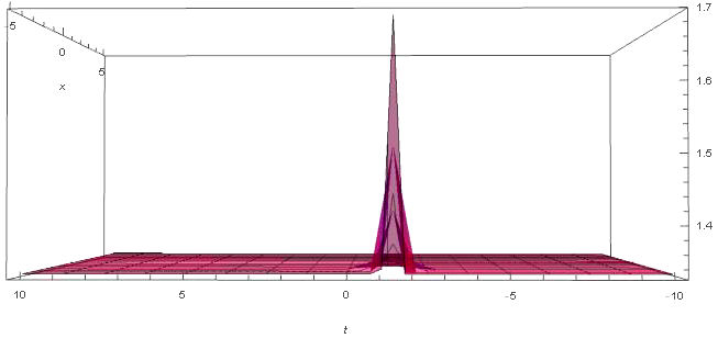
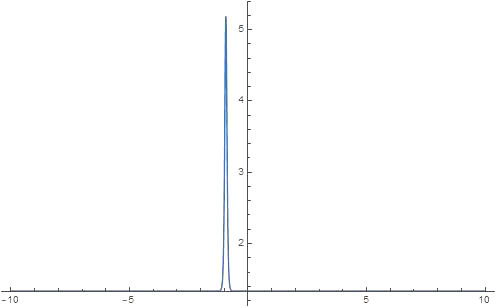
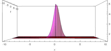
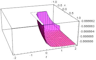
5 Concluding Remarks

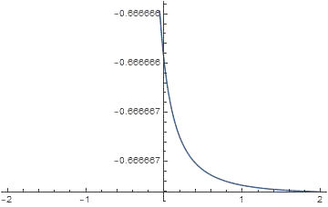
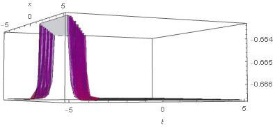
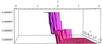
We have applied a new approach of the Kudryashov method to the time-fractional fifth-order Sawada-Kotera equation and the (4 + 1)-dimensional space-time fractional Fokas equation which arise in mathematical physics. The wave transformations applied with the help of beta derivative definitions and the Q function included in the algorithm facilitated the computation of the solutions. The general solutions for the time-fractional fifth-order Sawada-Kotera equation and the (4 + 1)-dimensional space-time fractional Fokas equation have been pointed out as polynomials of the logistic function, which in turn are solutions of the Riccati equation. Finally, some new exact solutions in the form of exponential functions for given equations are established. We have also presented the numerical simulations for equations thanks to three dimensional plots. Therefore, we conclude that this method may have general applications. As comparing the other methods, the advantage of this approach is that the form of function is not used at the calculation. This gives us not only ease of calculation, but also the opportunity to obtain new solutions. However, it should not be overlooked that this new method is more suitable for nonlinear equations with even-order derivatives. Hence, one can conclude that the method can method can be applied to many fractional partial differential equations.

References

1. I. Podlubny, Fractional Differential Equations. (Academic Press, 1999). [ Links ]

2. S.S. Ray, Nonlinear Differential Equations in Physics. (Springer, 2020). [ Links ]

3. S.S. Ray and S. Sahoo, A novel analytical method with fractional complex transform for new exact solutions of time-fractional fifth-order Sawada-Kotera equation. Rep. Math. Phys. 75 (2015) 63. https://doi.org/10.1016/S0034-4877(15)60024-6. [ Links ]

4. S.S. Ray and S. Sahoo, Two efficient reliable methods for solving fractional fifth order modified Sawada?Kotera equation appearing in mathematical physics. J. Ocean Eng. Sci. 3 (2016) 219. htts://doi.org/10.1016/j.joes.2016.06.002. [ Links ]

5. O.S. Iyiola, A numerical study of Ito equation and Sawada-Kotera equation both of time-fractional type. Adv. Math. Sci. Journal 2 (2013) 71. [ Links ]

6. M. Senol, L. Akinyemi, A. Ata and O.S. Iyiola Approximate and generalized solutions of conformable Type Coudrey-Dodd-Gibbon-Sawada-Kotera equation. Int. J. Mod. Phys.B 35 (2021) 2150021. htts://doi.org/10.1142/S0217979221500211. [ Links ]

7. P. Veeresha, H.M. Baskonus and W. Gao Strong Interacting Internal Waves in Rotating Ocean: Novel Fractional Approach. Axinoms 10 (2021) 123. htts://doi.org/10.3390/axioms10020123. [ Links ]

8. S. Zhang and H. Zhang, Fractional sub-equation method and its applications to nonlinear fractional PDEs. Phys. Lett. A 375 (2011) 1069. htts://doi.org/10.1016/j.physleta.2011.01.029. [ Links ]

9. H. Yepes-Martínez, J.F. Gomez-Aguilar and D. Baleanu, Beta-derivative and sub-equation method applied to the optical soli-tons in medium with parabolic law nonlinearity and higher order dispersion. Optik 155 (2018) 357. htts://doi.org/10.1016/j.ijleo.2017.10.104. [ Links ]

10. H.M. Baskonus and H. Bulut, Exponential prototype structures for (2+1)-dimensional Boiti-Leon-Pempinelli systems in mathematical physics. Wave in Complex and Random Media 26 (2016) 189. htts://doi.org/10.1080/17455030.2015.1132860. [ Links ]

11. R.M. Jena, S. Chakraverty, S.K. Jena and H.M. Sedighi On the wave solutions of time-fractional Sawada-Kotera-Ito equation arising in shallow water. Math. Meth. Appl. Sci. 44 (2021) 583. htts://doi/10.1002/mma.6763. [ Links ]

12. S. Sarwar, K.M. Furati and M. Arshad, Abundant wave solutions of conformable space-timefractional order Fokas wave model arising inphysical sciences. Alex. Eng. J. 60 (2021) 2687. htts://doi.org/10.1016/j.aej.2021.01.001g. [ Links ]

13. Y. Zhao and Y. He, The extended fractional DξαG/G -expansion method and its applications to a space-time fractional Fokas equation. Math. Probl. Eng. 2017 (2017) 8251653. htts://doi.org/10.1155/2017/8251653. [ Links ]

14. A. Dascioglu, S.C. Unal and D.V. Bayram, New Analytical Solutions for Space and Time Fractional Phi-4 Equation. MTU J. Eng. Nat. Sci. 1 (2020) 30. https://dergipark.org.tr/en/pub/naturengs/issue/54615/697242. [ Links ]

15. H. M. Baskonus, Complex surfaces to the fractional (2+1)-dimensional Boussinesq dynamical model with the local M-derivative. Eur. Phys. J. Plus 134 (2019) 322, https://doi.org/10.1140/epjp/i2019-12680-4. [ Links ]

16 . W. Gao, G. Yel, H. M. Baskonus and C. Cattani, Complex solitons in the conformable (2+1)-dimensional Ablowitz-Kaup-Newell-Segur equation. AIMS Mathematics 5 (2019) 507. https://doi.org/10.3934/math.2020034. [ Links ]

17. H.M. Baskonus, New acoustic wave behaviors to the Davey-Stewartson equation with power-law nonlinearity arising in fluid dynamic. Nonlinear Dyn. 86 (2016) 177, https://doi.org/10.1007/s11071-016-2880-4. [ Links ]

18 . F. Tascan, M. Kaplan and A. Bekir, Exponential rational function method for space-time fractional differential equations. Wave Random Complex, 26 (2016) 142, htts://doi.org/10.1080/17455030.2015.1125037. [ Links ]

19 . F. Meng, A new approach for solving factional partial differential equations. J. Appl. Math., 2013 (2013) 1, htt://dx.doi.org/10.1155/2013/256823. [ Links ]

20. Y. Gurefe, The generalized Kudryashov method for the nonlinear fractional partial differential equations with the beta-derivative. Rev. Mex. Fis. 66 (2020) 771. htts://doi.org/10.31349/RevMexFis.66.771. [ Links ]

21. S.T. Demiray, Y. Pandir and H. Bulut, Generalized Kudryashov method for time-Fractional differential equations. Abstr. Appl. Anal. 2014 (2010) 901540. htts://doi.org/10.1155/2014/901540. [ Links ]

22 . M. Bagheri and A. Khani, Analytical Method for Solving the Fractional Order Generalized KdV Equation by a Beta-Fractional Derivative. Adv. Math. Phys. 2020 (2020) 8819183. htts://doi.org/10.1155/2020/8819183. [ Links ]

23. S.M. Ege and E. Misirli, Extended Kudryashov method for fractional nonlinear differential equations. Math. Sci. Appl. Enotes, 6 (2018) 19. https://doi.org/10.36753/mathenot.421751. [ Links ]

24. E.M.E. Zayed et al., Cubic-quartic optical solitons with Kudryashov's arbitrary form of nonlinear refractive index. Optik 238 (2021) 166747, htts://doi.org/10.1016/j.ijleo.2021.166747. [ Links ]

25. Y. Yildirim et al., Highly dispersive optical solitons and conservation laws with Kudryashov's sextic power-law of nonlinear refractive index. Optik , 240 (2021) 166915. htts://doi.org/10.1016/j.ijleo.2021.166915. [ Links ]

26. D. Kumar, A.R. Seadawy and A.K. Joardar, Modified Kudryashov method via new exact solutions for some conformable fractional differential equations arising in mathematical biology. Chin. J. Phys., 56 (2018) 75. htts://doi.org/10.1016/j.cjph.2017.11.020. [ Links ]

27. Y. Yildirim et al., Cubic-quartic optical soliton perturbation with Kudryashov's law of refractive index having quadrupled-power law and dual form of generalized nonlocal nonlinearity by sine-Gordon equation approach. J. Opt. 50 (2021) 593. htts://doi.org/10.1007/s12596-021-00686-y. [ Links ]

28. E.M.E. Zayed, K.A. Gepreel, R.M.A. Shohib and M.E.M. Alngar, Solitons in magneto-optics waveguides for the nonlinear Biswas-Milovic equation with Kudryashov's law of refractive index using the unified auxiliary equation method. Optik , 235 (2021) 166602. htts://doi.org/10.1016/j.ijleo.2021.166602. [ Links ]

29. S. Sain, A.G. Choudhuryb and S. Garai, Solitary wave solutions for the KdV-type equations in plasma: a new approach with the Kudryashov function. Eur. Phys. J. Plus , 136 (2021) 226. htts://doi.org/10.1140/epjp/s13360-021-01217-1. [ Links ]

30. N. A. Kudryashov, Method for finding highly dispersive optical solitons of nonlinear differential equations. Optik 206 (2020) 163550, htts://doi.org/10.1016/j.ijleo.2019.163550. [ Links ]

31. N. A. Kudryashov, Solitary waves of the non-local Schrodinger equation with arbitrary refractive index. Optik 231 (2021) 166443, htts://doi.org/10.1016/j.ijleo.2021.166443. [ Links ]

32. R. Khalil, M. Horani, A. Yousef and M. Sababheh, A new definition of fractional derivative. J. Comput. Appl. Math. 264 (2014) 65, htts://doi.org/10.1016/j.cam.2014.01.002. [ Links ]

33. A. Atangana and D. Baleanu, New fractional derivatives with nonlocal and non-singular kernel: theory and application to heat transfer model. Therm. Sci., 20 (2016) 763, htts://doi.org/10.2298/TSCI160111018A. [ Links ]

34. A. Atangana and R.T. Alqahtan, Modelling the Spread of River Blindness Disease via the Caputo Fractional Derivative and the Beta-derivative. Entropy, 18 (2016) 40, htts://doi.org/10.3390/e18020040. [ Links ]

Received: June 24, 2021; Accepted: September 02, 2021

Creative Commons License This is an open-access article distributed under the terms of the Creative Commons Attribution License