


 nova página do texto(beta)
 Inglês (pdf)
 Artigo em XML
 Referências do artigo
 Enviar este artigo por email
 Citado por SciELO
  Similares em
SciELO
Similares em
SciELO 
 Permalink
1. Introduction
The model of an electron or some other particle confined inside a potential well of some shape, depth and volume is useful in many applications despite its simplicity. Examples of this include color centers in crystalline materials [1,2], quantum dots in nanotechnology [3,4], pi electrons in conjugated organic molecules [5] and electron bubbles in liquid ammonia or liquid helium [6-8]. Despite the confinement of the electron being a result of complex multi-particle interactions, the particle-in-a-box model often produces at least qualitatively correct results.
1.1. Potential wells with simple geometry
Often a real-world object can be modeled with some exceptionally simple physical system. An electron in a potential well with the shape of an exact cube or a sphere, and the potential energy V stepping abruptly at the well boundary is one example. In that situation, the potential energy of the electron is (spherical case)
or (cubic case)
Here the V 0 is the depth of the well. Θ is the Heaviside theta function,
ρ is the radius of the circular or spherical potential well and
L is the side length of the cubic potential well. The
variable r is just the distance from the origin in 2D or 3D
space:
Here x is a two- or three-dimensional vector.
1.2. Lamé circles and spheres
In real-world situations it can not always be assumed that the electron is confined to an exactly spherical or cubic space. The choice V 0 = ∞ is another crude approximation. A logical improvement to the model would be to define 2D curves and 3D surfaces with a shape between a square and a circle or cube and a sphere. One geometrical object of this type is the Lamé circle (or supercircle)
and the Lamé sphere (or supersphere)
Yet another name for these curves and surfaces is superquadrics. The objects described by these equations, with α = b = c = 1 (as in all cases studied in this article), become a circle or sphere when q = 2 and a square or a cube when q → ∞. The parameter r > 0 is the radius of the circle or sphere that these shapes become when q → 2. As a general result, an n-dimensional solid of this shape has volume [9]
where Γ is the gamma function. To produce a set of surfaces described by (6),
having different values of q but same constant enclosed volume
or the equivalent for a 2D Lamé circle.
3D surfaces of shapes given by Eq. (6) with α = b = c = 1 are shown in Fig. 1.
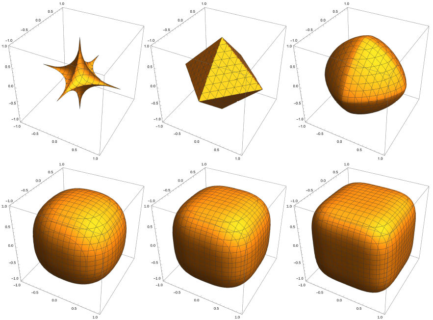
FIGURE 1 Wolfram Mathematica 11.2.0 plots of the surface defined by |x| q + |y| q + |z| q = r q for values q = 0.5, q = 1.0 q = 1.5, q = 2.5, q = 3 and q = 4 from left to right and up to down. The parameter r has been set to value 1.
The system with a potential well bounded by a Lamé curve has been studied earlier by Bera et al. [10], but only for the 2D case and with infinite V 0. In this article, the results will be extended to the equivalent 3D systems with several finite values of V 0 allowed.
A similar method of analytical geometry exists for converting a sphere continuously into a Platonic solid (regular octahedron, dodecahedron or icosahedron instead of a cube) [11,12], and it can be expected that the energy eigenvalues of an electron in that kind of potential well approach the spherical case when more faces are added to the polyhedron.
1.3. Experimental methods
A practical system that can be modelled as one or more electrons in a 1 to 3-dimensional potential well is the quantum dot (QD), which is a nanometer-scale semiconductor particle having an absorption/emission spectrum similar to a system of electrons confined in a potential well of equivalent size. An electron in a large QD has a lower ground state energy than one in a small QD, just like an electron in a short versus long 1D square well. One complication in this theory of QDs is the -possibly position-dependent- difference of electron and hole effective masses to their normal value or the value in bulk semiconductor [13]. This kind of nanoparticles can be produced by chemical or mechanical means such as molecular beam epitaxy or chemical vapor deposition [14], and their shape can be probed by methods such as measuring their spin and parity oscillations in a magnetic field [15]. Information about the effect of shape changes, as in the model systems of this article, on the electronic spectrum of the system can also be utilized for quantum dot shape determination. Conversely, this also means that QDs with desired spectral properties can be produced by tuning their shape in an appropriate way.
1.4. Computational approach
The methods applied in this article are numerical, with ground state and first excited state energies obtained with quantum diffusion Monte Carlo (QDMC) or Implicit finite differencing (IFD) on imaginary time axis. The system is a 2D or 3D potential well with boundary described by Eqs. (5) and (6). The parameters α, b and c all have value 1 , so the well is not oblong in any particular direction. The system contains one or two confined electrons. A suitable nonlinear fitting function is sought for the data points of ground state energy E 0 as a function of q and V 0. This is done to make it easier to estimate the E 0 for other values of q, V 0 by interpolation. With spectroscopic data and these results, it may be possible to estimate whether an electron-trapping cavity in a real material is more close to sphere or cube in shape.
Both the QDMC and IFD methods for finding the ground state are based on the time
evolution of an initial state |Ψ(0)⟩= c
0|ψ
0⟩ + c
1|ψ
1⟩ + c
2|ψ
2⟩... written as a linear combination of the
eigenstates of
Here it is assumed that
Provided that the E
n
form an increasing sequence of positive numbers, the state vector
|Ψ(τ)⟩ of (10) approaches something proportional to
|ψ
0⟩ when τ → ∞. This allows the numerical calculation
of the ground state wave function ψ
0(x) = ⟨x| ψ
0⟩. The eigenvalue E
0 can be obtained by following the expectation value
The difference between the QDMC and IFD methods is that in QDMC the diffusive imaginary-time dynamics is modelled as a system of random walkers with a source term allowing creation and destruction of them. The IFD method calculates actual wave functions that do not have to be real and positive valued.
2. Numerical methods
The diffusion Monte Carlo calculation was done with a C++ source code described in
[16] and appropriately modified to fit
this particular problem. The code utilizes atomic-like units with Planck constant
and electron mass set to
2.1. Transcendental equation and shooting method for q = 2 and q = ∞
2.1.1. Solution with non-algebraic equations for q = 2 and q = ∞
The calculation of the energy eigenvalues for a finite square, cubic or spherical potential well is described in most basic QM textbooks such as [17]. The method is based on the graphical solution of a non-algebraic (transcendental) equation. For a 1D square well with potential energy
the equation is
for the even states such as the ground state, and
for the odd states like the 1st excited state. The quantities α and β are defined as
These equations can be solved graphically after a straightforward conversion
to units where
The equation for solving energy eigenvalues of a 3D spherical potential well,
is of form
with
However, Eq. (16) is only for rotation invariant eigenstates with zero angular momentum, of which the ground state is one example. For numerical work, these quantities have to be made dimensionless and shifted to make the interior of the potential well have V = 0 as defined in this article.
2.1.2. Shooting method
For the 2D circular potential well, the corresponding equation contains special functions, and the result can more easily be obtained with the shooting method for the L = 0 eigenstates. The Schrödinger equation can be cast into polar coordinates
which simplifies for the rotation invariant ground state
The equation above can be solved numerically by changing to dimensionless variables and choosing a trial value of E and a small number ( << 1. Then it is integrated by finite difference starting from r = ( (not r = 0, to avoid problems with the singular multiplier 1/r in the polar Laplacian) with initial conditions ψ(() = 1 and ψ ’(() = 0. The value of E is adjusted until the radial wave function doesn’t blow up to negative or positive infinity near the potential step r = ρ. The smallest value of E with this property can be taken as an approximation for E 0. The same procedure can also be applied for finding the energies E n of other rotation invariant eigenfunctions of the Hamiltonian, but the first excited state with energy E 1 is not one of those.
2.2 Quantum DMC for one particle in 2D and 3D
The diffusion Monte Carlo results for both 2D and 3D were calculated with values of 2 ≤ q ≤ 20 and 50 ≤ V 0 ≤ 20000.
The result for each combination of q and V 0 was calculated 4 times and averaged to one data point. The time step length in both 2D and 3D simulations was ∆t = 10−5, the energy update parameter was α = 40 and the maximum allowed number of random walkers was 105 (2D) or 9 × 10⁵ (3D). Simulated time length was 20 units, and 1/4 from the beginning of the energy output file was discarded before averaging the remaining energy values to an estimate for E 0.
The results were plotted as graphs where either V 0 or q was kept constant and the other varied. Particle mass was set to 1 in all calculations. The area of a 2D potential well was kept constant at A = 4 when changing the value of the exponent q, and the volume of the 3D potential well was kept at V = 8. This was done by defining r = r(q) as in (8).
Calculations for well depths of 600, 2000 and 20000 were also done similarly for
a 3D well of volume
In preliminary calculations, it was seen that an exponential function of type
fits well in the data points of E 0 as a function of q, and a rational square root function
to the data points of E 0 as a function of V 0. Making Eq. (20) more complex by converting it to a sum of two exponentials did not add any more accuracy in the fit. Both kind of graphs (as a function of q or V 0) can be used for estimating the ground state energy for intermediate values of q and V 0 by interpolation. There is no obvious theoretical reason for the E 0(V 0) and E 0(q) to be close to these functions; the reason for calculating the nonlinear fit is just to predict the behavior of the functions between calculated data points.
The results were plotted and the iterative nonlinear fits calculated with the Linux application Grace-5.1.25. The obtained values of fitting parameters A 0, A 1 and A 2 were recorded for all cases. Another way to do the curve fit is to fix A 0 and A 1 to values predicted by a transcendental equation or with the shooting method, and leave only A 2 free.
2.3. Quantum DMC for two particles in 2D
2.3.1. Basic parameters
The problem of two electrons in the same potential well was numerically investigated only in 2D to limit the computation time. Instead of having only q and V 0 as parameters, the area of the potential well was also varied to see its effect on E 0. The maximum number of random walkers in these simulations was 30000 and the time step was 3×10⁻⁶. The energy update parameter α needed to have higher value, up to 120, than in the 1-particle version to give better accuracy.
The value of q in these results was either 2, 8 or ∞. The well depth was V 0 = 200 or 20000. The size of the potential well was parametrized with a variable s, with the area of the potential well being π when s = 1 and πs 2 for other values of s. In other words, s is a multiplier of all linear dimensions of the system. The parameter s was varied from s = 1 to 4 in steps of 0.5. In addition to the ground state energy E 0, the mean electron-electron distance r 12 was extracted from the output wave function.
2.3.2. Electron-electron interaction energy
The position representation Hamiltonian of two interacting electrons confined in a supercircular potential well is
where the
A system of only two electrons does not require any special care to antisymmetrize the ground state wave function, because the two electrons can have opposite spins.
2.4. Implicit finite-differencing for one particle in 2D
2.4.1. Description
In the simplest possible case of a 1D quantum system, the time-dependent
Schrödinger equation is made discrete by replacing the wave function
Ψ(x,t) with an array
As described in [19], the
Crank-Nicolson method is a way to turn the discrete
version of the Schrödinger equation into an implicit scheme that preserves
unitarity. This is done by approximating the evolution operator
where the units have been chosen so that
If the operator
With V
j
the array of position-dependent potential energy values. This is a
tridiagonal system of linear equations for solving the array
2.4.2. 2D systems
In the 2D case, the discrete object replacing the wave function
Ψ(x,y,t) is a three-index array
Here it is assumed that the spatial step size is the same ∆x
to both x and y directions. However, this
equation cannot be written as a tridiagonal system anymore, and this makes
the computational cost of the problem increase very rapidly with increasing
size of the discrete x-y grid. More specifically, the number of arithmetic
operations needed for solving a tridiagonal system of n
equations and n unknowns scales as
2.4.3. Operator splitting
One way to circumvent this problem for large discrete systems is to approximately divide every time step to three parts. In the first part, the x-direction kinetic energy is accounted for by solving
The second equation is the same for y-kinetic energy:
and the third equation is just a multiplication with a complex phase factor
The justification of doing this is that for ∆t << 1,
the evolution operator
despite
Both (27) and (28) can be written as tridiagonal matrixvector equations, and the multiplication (29) is a trivial calculation. The time step ∆t has to be smaller than when solving the dynamics from (26), but this operator splitting method still produces a significant increase in computational speed for large grids of points (j,k). This operator splitting method and its modifications have been used, for instance, in [20] in the context of wavepacket dynamics and in [18] to factorize operators in quantum statistical mechanics.
2.4.4. Simulation parameters
In the actual simulations, the domain in xy-plane was a square with opposing corners at (0,0) and (3.4,3.4). This domain is large enough to contain any potential well of area 4.0 and shape given by (5) with 2 ≤ q < ∞. Enough grid points are also left outside the well for the wave function to practically reach zero before the boundaries of the domain (given that the depth of the well is V 0 ≥ 2000). The center of the potential well is at (x,y) = (1.7,1.7), and the spatial discretization contains 850 × 850 points. The function “Solve.tridiag” from the limSolve package was used for solving the linear systems in R.
The time step was ∆t = 10−4 in all cases, and the
simulation length on imaginary time axis had to be t
max
> 1.5 for good convergence. Once the
ground state quantities E
0 and ⟨x|ψ
0⟩ were calculated by this scheme, the 1st excited state was
obtained in the same way with the ground state component removed from Ψ on
each time step with projection:
The initial state
The eigenvalues E 0 and E 1 were calculated for V 0 = 2000 and V 0 = 20000, and for all values of q from the set {2,4,6,8,10,15}. After all data points E 0(V 0 ,q) and E 1(V 0 ,q) were obtained, the function (21) was fitted to all result sets.
In addition to that mentioned above, the 2nd excited state energy E 2 was calculated for the q = 2 case with both V 0 = 2000 and V 0 = 20000. This was done by doing another simulation where the wave function was orthogonalized with both |ψ 0⟩ and |ψ 1⟩ on each time step. The reason for calculating this was that the first excited state |ψ 1⟩ and its energy eigenvalue E 1 can’t be obtained by the shooting method, because it is not rotation invariant. Comparison of the E 2 from IFD integration to the value solved with Eq. (19) is one way to verify the correctness of the IFD method applied here.
3. Results
3.1. Ground state energy of q = 2 and q = ∞ potential wells
The results for the E 0 of square/cubic systems with side length 2, obtained from the graphical solution of Eq. (12), are on the left side of Table I.
TABLE I The ground state energy, E0 of a particle of mass 1 in a 2D or 3D potential well with q = ∞ (left table) or q = 2 (right table), area 4.0 and height of potential barrier V0.
| V0 | E0 (square) | E0 (cube) | E0 (circle) | E0 (sphere) |
| 50 | 2.0380 | 3.0570 | 1.9140 | 2.7146 |
| 100 | 2.1518 | 3.2277 | 2.0102 | 2.8679 |
| 200 | 2.2378 | 3.3567 | 2.0821 | 2.9617 |
| 600 | 2.3308 | 3.4962 | 2.1591 | 3.0616 |
| 1200 | 2.3696 | 3.5544 | 2.1911 | 3.1028 |
| 2000 | 2.3912 | 3.5868 | 2.2087 | 3.1256 |
| 10000 | 2.4328 | 3.6492 | 2.2428 | 3.1696 |
| 20000 | 2.4430 | 3.6645 | 2.2511 | 3.1801 |
The equivalent results for 2D circular or 3D spherical potential wells, with area 4 or volume 8 are shown on the right side of Table I. The former has been obtained with the shooting method and the latter with Eq. (16).
3.2. QDMC results for one particle in 2D or 3D
For both 2D and 3D, and for every value of V
0 from 50 to 20000, 12 ground state energy data points from
q = 2 to q = 20 were obtained in the QDMC
calculation. To each point set of different V
0, the exponential function of (20) was fitted to the
E
0(q) data. This was done both with all parameters
A
0, A
1 and A
2 free, or with A
0 and A
1 fixed to the limiting values of E
0(q = 2) and E
0(q → ∞) for that V
0 (Table I) and only
A
2 left free. Figures 2 and 3 show both the E
0 data points and the 1- or 3-parameter curve fits to the data with a
potential well of area A = 4.0 or volume
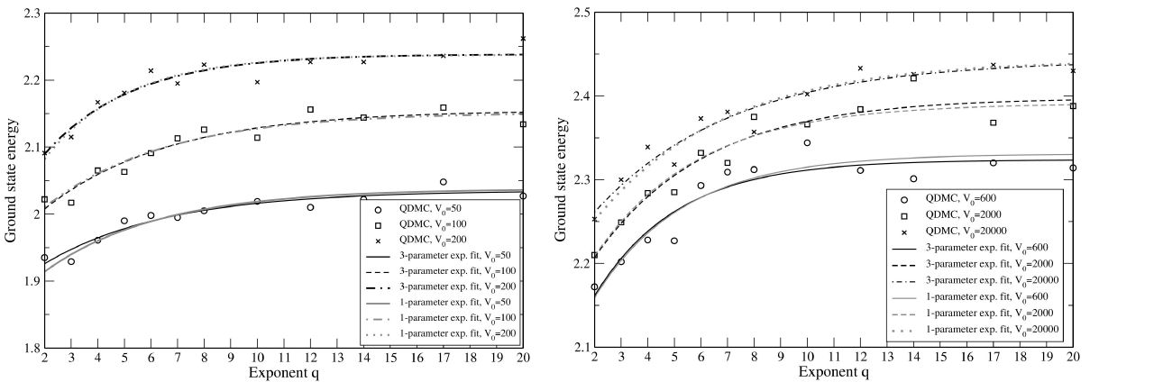
FIGURE 2 QDMC ground state energies and 1- or 3-parameter exponential
curve fits (20) for one electron in a 2D potential well of shape (5)
and area 4.0, and with different values of exponent
q. The units have been chosen so that
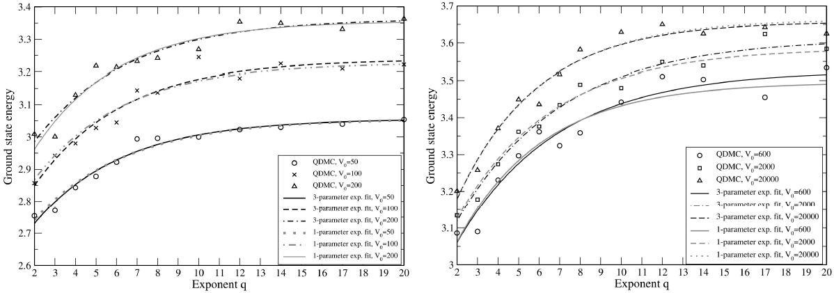
FIGURE 3 QDMC ground state energies and 1- or 3-parameter exponential
curve fits (20) for one electron in a 3D potential well of shape (6)
and volume 8.0, and with different values of
exponent q. The dimensionless units are again
The similarity of the 1-parameter (gray lines) and 3parameter (black lines) exponential fits in Figs. 2 and 3 reflects how accurately the E 0 values calculated with QDMC agree with those calculated by different means for the q = 2 and q = ∞ limiting cases (Table I).
Main important features in the data of Fig. 2 and 3 include that the E 0 grows monotonically with increasing q in all cases, and the difference in E 0 between q = 2 and q = ∞ is in the range of 5-15%. Most of the change in ground state energy in all data sets has already taken place when q has increased to value 8 from the original 2. The nonlinear fit parameter A 2 was between −0.30 and −0.20 for almost all data sets.
Figure 4 shows the additional results E 0(q) for the three cases of a 3D potential well of smaller volume 2.0. The graphs look similar to those for larger potential wells, except for the E 0 values being higher. The curve fit parameters of Figs. 2 to 6 are also included as tables of numerical data in the Appendix.
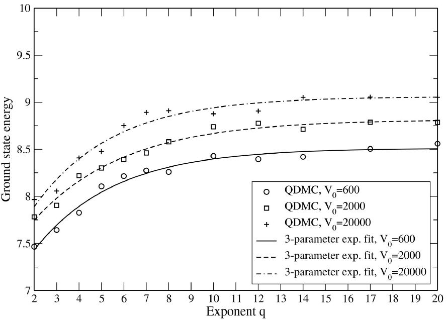
FIGURE 4 QDMC E 0 values and 3-parameter exponential curve fits (20) for one electron in a 3D potential well of shape (6) and volume 2.0, and with exponent q as the independent variable.
It is also possible to present the data as graphs with q and
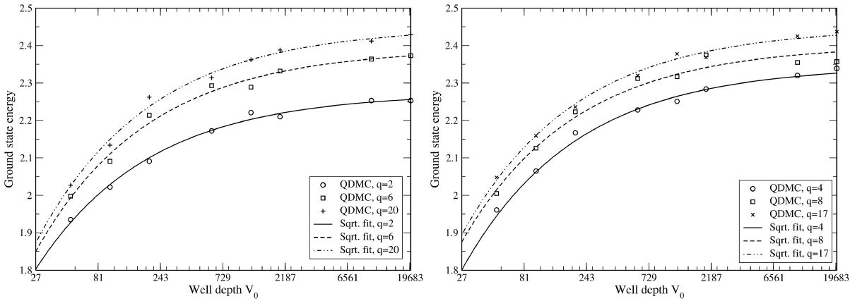
FIGURE 5 QDMC ground state energies of one electron as function of V 0 for a supercircular potential well of area 4.0, shape given by Eq. (5) and several values of exponent q. The square root type curve fits of Eq. (21) are also shown in the figure.

3.3. QDMC results for two particles in 2D
The QDMC ground state energies, E
0, for two interacting or non-interacting electrons in a 2D potential
well of depth V
0 = 200 or V
0 = 20000 are shown in Fig. 7
with the value of parameter s varying from 1.0
to 4.0. The area of the potential well is A =
π when s = 1 regardless of what the value
of q is and A = πs
2 for other values of s, to make the results easier
to compare. For q = 2 it holds that s =
r, for q = 8 the relation is
s ≈ 1.1162r and for
q = ∞, s ≈
1.1284r with r as in Eq.
5. More generally, for a given value of q and 2p-dimensional
space the connection between s and r is
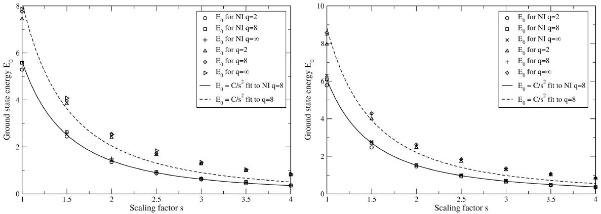
FIGURE 7 QDMC ground state energy E 0 for two interacting or non-interacting (NI) electrons in a supercircular potential well of depth V 0 = 200 (left) or V 0 = 20000 (right). The parameter q is the same as in Eq. (5) and s a linear scaling factor, with the area of the supercircle being πs 2 for a given value of s. An E 0(s) ∝ s −2 nonlinear fit has been made to the q = 8 data points to demonstrate the difference caused by the presence of Coulomb interaction.
In the graphs, there is also a curve fit of form E 0(r) ∝ r −2 made for each q = 8 data point set. The energy eigenvalues of a set of non-interacting particles, in a potential well deep enough for approximation V 0 = ∞ to be valid, are proportional to reciprocal square of the well diameter. From Fig. 7 it is easy to see that this type of function can be quite accurately fitted to the q = 8 data points for noninteracting electrons, even for the lower well depth V 0 = 200, but not accurately at all to the point sets with Coulomb potential included.
The expectation values hr 12i are shown as function of s for potential wells of both depths in Fig. 7. Parabolas ⟨r 12⟩ (s) = c 2 s 2 + c 1 s + c 0 have also been fitted in each set of data points, and the result is that each point set is close to being on the same line with |c 1| > 50|c 2|.
The effect of making the parameter ( (meant to prevent division by zero when
calculating the electron-electron Coulomb potential) smaller by a factor of 100
was also tested in the q = 2, V
0 = 200 case with two interacting electrons. Figure 8 shows how much difference this causes in the
E
0(s) data points. The value ( =
0.001 may look large, especially when it’s inside the
square root in
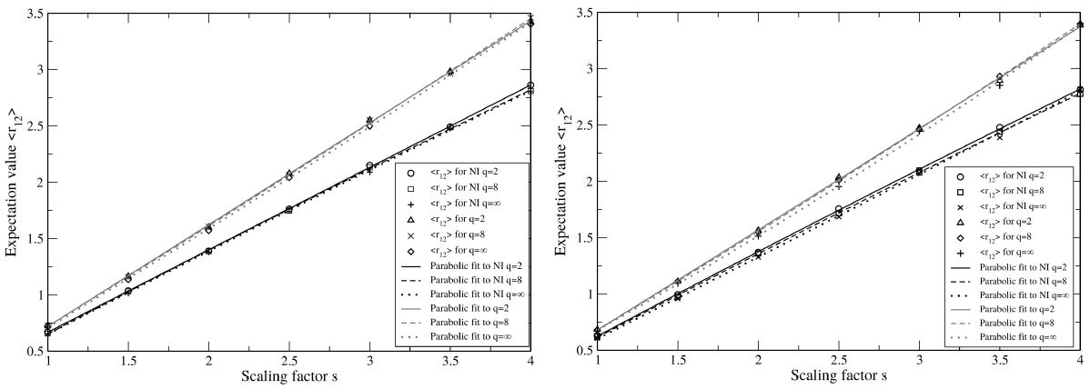
FIGURE 8 QDMC expectation values hr 12i for two interacting or non-interacting (NI) electrons in a supercircular potential well of depth V 0 = 200 (left) or V 0 = 20000 (right), parameter q as in Eq. (5) and s a linear scaling factor such that the area of the supercircle is πs 2 for a given value of s.
The Appendix contains the tables of numerical data for E 0 (Fig. 7) and ⟨r 12⟩ (Fig. 8) as a function of r and for different well depths.
3.4. Implicit time stepping results for one particle in 2D
When exponential functions of type (20) were fitted in the E 0 and E 1 values obtained with the IFD method and imaginary time propagation, the parameters A 0, A 1 and A 2 of Eq. (20) were found to be as in Table II. The data points E 0(q) and E 1(q) are shown with the nonlinear fits in Fig. 10.
TABLE II The parameters A0, A1 and A2 of (21), with the nonlinear fit done to E0(q) and E1(q) values obtained with finite difference imaginary time propagation for a single electron in a 2D potential well of area 4.0, depth V0 and shape given by (5).
| eigenvalue | A0 | A1 | A2 |
| E0 (V0 = 2000) | 2.3896 | 2.2072 | -0.25035 |
| E1 (V0 = 2000) | 5.9779 | 5.6029 | -0.22288 |
| E0 (V0 = 20000) | 2.4366 | 2.2448 | -0.25274 |
| E1 (V0 = 20000) | 6.0957 | 5.6985 | -0.22526 |
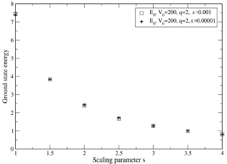
FIGURE 9 The values of E 0(s), obtained with QDMC, for two interacting electrons in a potential well with q = 2 and V 0 = 200 and with two different values of cutoff parameter (.
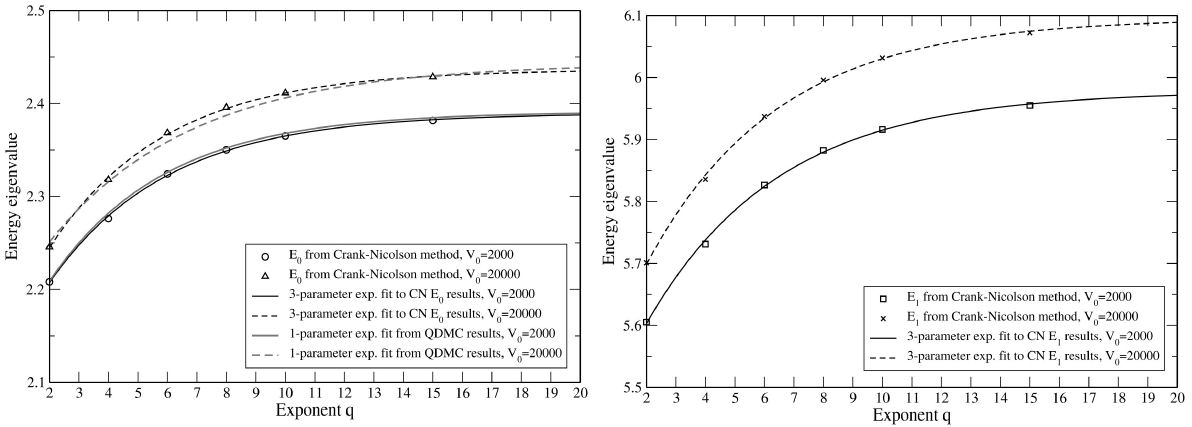
FIGURE 10 Energy eigenvalues E 0 (left) and E 1 (right) for one electron in a 2D potential well of shape (5), area 4.0 and depth V 0 = 2000 or V 0 = 20000. The results were calculated by imaginary time propagation done with implicit finite differencing and operator splitting. In the left image, the equivalent QDMC results are also plotted for comparison.
The A 0 values (limit of E at q → ∞) for the ground states of V 0 = 2000 and V 0 = 20000 are 2.3896 and 2.4366. When these are compared to values in Table I, 2.3912 and 2.4430, the error in the first case is less than 0.1% and that in the second, less than 0.3%. The corresponding ground state A 1 values are 2.2072 and 2.2448, representing the limit of E 0 for q → 2. The equivalent values in Table I, calculated with the shooting method, are 2.2087 and 2.2511. The difference between the IFD and shooting method values is less than 0.3% in both.
The A 0 values for the first excited state, calculated with IFD method, were 5.9779 and 6.0957. The 1st excited state energy E 1 can also be calculated for the q → ∞ system with Eqs. (12) and (13), and the results for V 0 = 2000 and V 0 = 20000 are 5.9779 and 6.1073. The differences between the IFD results and those from (12) and (13) are here less than 0.2%.
The value for the second excited state energy E 2 from the IFD simulations done for q = 2 case were 11.6338 for V 0 = 2000 and 11.8318 for V 0 = 20000. When a shooting method calculation was done for these two systems with a rotation invariant 2nd excited state, the results were 11.635 for V 0 = 2000 and 11.861 for V 0 = 20000. Here the percentual error is again less than 0.3%. The consistency between q = 2 and q = ∞ results obtained with different methods makes it seem likely that the results of Fig. 10 are close to correct also for values of q between the two extremes.
4. Conclusion
In this work, the ground state energies of potential wells of Lamé circle or Lamé sphere shape were calculated for a large number of combinations of well depth V 0 and the exponent q in Eq. (6). In most calculations the parameter r of (6) was defined as a function of q, r := r(q), to keep the area or volume of the potential well at a q-independent constant value. It was also shown that simple functions of 2 or 3 parameters can be accurately fitted in the E 0(q,V 0) data points, but there is no obvious way to show mathematically that the function E 0(q) could be written as a sum of an exponential plus small correction terms. Based on the more accurate data points in Fig. 10, it does not even seem completely impossible that the exponential dependence of E 0 on q with V 0 and V kept constant could be the exact solution of the problem.
The most surprising fact in this was that the multiplier A
2 in the optimal exponential function fit seemed to have a similar value
of −0.30 ≤ A
2 ≤ −0.20 for all well depths, volumes and both in 2D
and 3D. Furthermore, most of the variation in the value of that parameter appeared
to be random numerical error, because the value didn’t consistently change to either
direction when the well depth or volume was altered. The variation in those values
was greater for the 2D potential wells for which the calculations were done with a
smaller number of random walkers. A simple back-of-the-envelope way to approximate
the E
0 for some V
0,
In the case of 2D potential wells, calculations were also made for the first excited state energy E 1 of one electron, and the ground state energy E 0 and expected electron-electron distance ⟨r 12⟩ of two electrons confined in a 2D Lamé circle. The value of ⟨r 12⟩ was found to increase almost linearly as a function of a scaling parameter s.
In the cases where it was possible to compare results calculated by different means for the same system, there was a good agreement between QDMC, IFD imaginary time propagation, shooting method and graphical solution results. Especially the consistency of the QDMC and more accurate IFD results in the left image of Fig. 10 is a good sign that the 2D QDMC results are correct enough despite the significant random error in individual data points (Fig. 2).
The results are an extension of those in Ref. [10], where only 2D potential wells of infinite depth were considered. As remarked in that publication, this kind of results can be used for estimating the cube- or spherelikeness of a real physical potential well system, such as an electron in a quantum dot or a vacant site of a crystal lattice. Another possible application of the content of this article could be as an example problem for students of computational chemistry and physics.
One problem related to the material in this article is the behavior of two oppositely charged particles in a 2D or 3D potential well. This could be described as a hydrogen atom [21, 22] or positronium [23] being compressed by an external force, and the interparticle distance hr 12i would approach some finite limiting value with increasing scaling parameter s.
It has probably been known since the early years of quantum mechanics that a system of a particle interacting with a 3D spherical potential well doesn’t necessarily have even one bound state, while one in a rectangular potential well always does. The existence of a bound state in the spherical well depends on whether its V 0 and radius are large enough. One unanswered question is whether there exists some finite minimum value of the exponent q in Eq. (6) that guarantees the existence a bound state for a potential well with that bounding surface. One possible way to heuristically probe the situation would be to add more data points of low V 0 to the data in Figs. 5 and 6 and extrapolate to V 0 → 0, but an actual mathematical proof would be a completely different task.

