


 nova página do texto(beta)
 Inglês (pdf)
 Artigo em XML
 Referências do artigo
 Enviar este artigo por email
 Citado por SciELO
  Similares em
SciELO
Similares em
SciELO 
 Permalink
1. Introduction
The search for new physics and standard-model tests in high energy physics, more than ever, demands the exploration of highly sophisticated processes [1-8]. This brings along experimental challenges as, for example, the implementation of multiparticle detection and measurement. In this context, the theoretical study of the spin-dependent observables and the analysis of high-order processes require the calculation of transition amplitudes of increasing complexity. Because these amplitudes involve a large number of Dirac particles, coupled through interaction terms with several gamma matrices [9-12], the textbook methods become cumbersome to calculate with.
The algebraic structure of physical amplitudes demands the use of bold and clever methods to provide an analytical value. Modern techniques for amplitude calculation have been improved, especially for interactions with many particles [13-16], and are usually optimized for some computational implementations [17-20]. However, almost all of these techniques are devoted to helicity states for fermions [21-29] and only a few can be regarded as an analysis tool for general spin directions [30].
Our goal in this work is to develop a fully covariant method which allows obtainong efficient and compact analytical expressions for the spin-dependent amplitude, so that the framework can be employed within a computational program. Also, we want to suggest that a simple unifying framework to many other approaches can be formulated with our expressions.
The organization of this work is as follows. Section 2 sets the basic notation and contains the central idea of our procedure: the covariance of Dirac spinors and its implications to the closure property, along with the decomposition of an operator in terms of spinors. Section 3 presents a systematic framework for spin amplitude calculation, we call this scheme the projective method. The method is exemplified using the spinor rest frame basis. Section 4 is devoted to formulate the massless-spinor method [18] using the structures of the Sec. 2. In Sec. 5, it is shown that the helicity-spinor method can also be structured within this framework. We give an example of all of these procedures by computing the Compton Scattering amplitude in Sec. 6. Finally, Sec. 7 contains the conclusions. Bjorken and Drell [31] notation and units will be adopted throughout this text.
2. Completeness of the Dirac spinors
The Dirac equation for a free particle of mass m
 (1)
(1)
where e = ±1 is the sign of the energy (Ref. 31, pag. 28), uses two different representations of the Lorentz group. On one hand, the four-vector operator
where x
μ
= (t,
The operator  contains the Dirac matrices γ
μ
which, due to the Lorentz invariance of the Dirac equation (1), transform as both spinor and four-vector object. To fully appreciate what this implies, it is useful to recall the properties of a Dirac spinor.
contains the Dirac matrices γ
μ
which, due to the Lorentz invariance of the Dirac equation (1), transform as both spinor and four-vector object. To fully appreciate what this implies, it is useful to recall the properties of a Dirac spinor.
The spinors u(p, ±s) and v(p, ±s) satisfy the set of eigenequations
 (3)
(3)
and form a complete basis for any four-component spinor, i.e. an arbitrary Dirac spinor w, with four-momentum p׳, four-spin s' and mass m׳ can be expanded in the form
where it is used the notation
The expansion (4) will not mix spinors of opposite energy if it connects spinors with the same four-momenta. This means that the representation of u(p, s
'
) or v(p, s
'
) will only have non-zero terms for coefficients
The orthogonality between spinors u (p, s) and v (p, s
'
) is evident in their rest reference frame, where the Dirac spinors of different energies are mutually orthogonal, no matter which spin directions are chosen. Using a Lorentz transformation S (
is evident and shows that it will hold in any reference frame. Also, formula (4) can be proven by taking advantage of its fully covariant structure, as it is noticed in (Ref. 31, pag. 31), and this suggests that its use will, in turn, generate covariant expressions.
The transformation rule of Dirac matrices (Ref. 31, pag. 20), can be further appreciated with the insight that equation (4) provides. Using it, one can demonstrate the expansion
where r,r' = 1,2,3,4, the spinor 𝜔
r
(Q,S) = u(Q, (-1)
r+1
S), for r = 1,2; and 𝜔
r
(Q,S) = v(Q, (-1)
r
S), for r = 3,4. Expression (6) shows a twofold composition of representations of the Lorentz group. While the coefficients
A general spinorial operator O will be covariant if it transforms under the Lorentz group as O' = S O S-1. If O is written as
the covariance is verified if the s, p, v μ , a μ and Ω μν are objects that transform under the four-vector representation as a scalar, pseudo-scalar, vector, axial-vector, and tensor quantities, respectively. If a covariant operator acts upon any spinor 𝜔 r (Q), a new spinor O 𝜔 r (Q) is obtained. In general, this spinor is not necessarily an eigenstate of Eqs. (3), but the result can be expressed as a linear combination of a complete spinorial basis. This idea will be extensively used in the following sections, but the relevance of the completeness in the spinor space becomes now clear.
In the next section, the expressions (4) and (6) will be used to compute a general Dirac amplitude, and that will enable us to understand other techniques systematically.
3. Projective method for the amplitude computation: a General Framework
A Dirac amplitude is a matrix element of the, usually, covariant operator Γ. Its Lorentz scalar nature is revealed when one looks at its explicit form. For example, with positive energy states, it looks as
The main purpose of the spinorial techniques is to obtain the analytical value of expression (8) in terms of simple elements, such as inner products between four-vectors, or the volume subtended by four-vectors ε αβγδ a a b ß c γ d δ (where ε0123 = +1 is the Levi-Civita symbol of four indices). A common trick is to rewrite Eq. (8) as
This procedure has the advantage of explicitly displaying the two covariant objects that constitute the amplitude. Furthermore, using the trace properties of gamma matrices it is possible to obtain an analytical expression for the amplitude. While the Γ operator is usually given in the representation that is shown in Eq. (7), the operator u(p, s)
3.1. The rest basis
In the rest frame of the Dirac spinors, we rewrite Eqs. (3) as
 (10)
(10)
with the spinors at rest Փ11( ) = S() = S( ) = S() = S(
 μ = (1/ιη)
Λμν(μ
= Λμν(
μ = (1/ιη)
Λμν(μ
= Λμν( ). The Matrix Λ(
It is easy to see that the representation of the Dirac spinors in (Ref. 31, pag. 30) allows for a projective decomposition of the Dirac spinors in terms of the spinors at rest
Note that expressions (11) are easily derived using the standard gamma-matrices representation (Ref. 31, pag. 30). They remain valid in an arbitrary representation since two sets of gamma matrices, γμ and γμ, are equivalent under similarity transformations ([35]).
Using expressions (11), Eq. (9) takes the form
 (12)
(12)
where both particles can have different masses and the operator Ραβ(p,s) = Π(α,p)
Σ (β, s) = = Σ(β,s) Π(a,p) is constituted with Π(α,p) = (α  +
m)/2m and Σ(β,s) =
(βγ
5
+
m)/2m and Σ(β,s) =
(βγ
5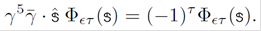 +
1)/2, the energy and spin projectors, respectively, pertaining to positive spin
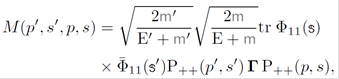
and energy for α = β = +1. A transition amplitude for a process
between an initial spinor of energy sign α = (-1)
𝜖+1 and spin eigenvalue in the frame at rest (-1)
𝜖+𝜏 = β(-1) 𝜖+1 and a final spinor
of energy sign a' = (-1) 𝜖´+ 1 and spin eigenvalue
in the frame at rest (-1) 𝜖´+ 𝜏´ = β´(-1)
𝜖´+ 1 is written as
+
1)/2, the energy and spin projectors, respectively, pertaining to positive spin
and energy for α = β = +1. A transition amplitude for a process
between an initial spinor of energy sign α = (-1)
𝜖+1 and spin eigenvalue in the frame at rest (-1)
𝜖+𝜏 = β(-1) 𝜖+1 and a final spinor
of energy sign a' = (-1) 𝜖´+ 1 and spin eigenvalue
in the frame at rest (-1) 𝜖´+ 𝜏´ = β´(-1)
𝜖´+ 1 is written as
(13)
To be useful, the expression in (13) needs the operator expansion of
Փϵτ ( ) ')
in terms of equation (7). The task is simple compared to the work required to
compute u(p, s)
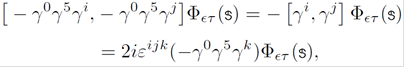
This can be seen from the spin equation in (10)
(14)
Equation (14) implies, via the eigenvalue equation
γ0Φετ() =
-(-1)𝜖Φ𝜖𝜏(), that the spinors Ф𝜖1 ( ) and Փ𝜖2 () are eigenstates of the
operator  = with eigenvalues
-(-1)𝜖/2 and +(-1) 𝜖/2 respectively. Operators
= with eigenvalues
-(-1)𝜖/2 and +(-1) 𝜖/2 respectively. Operators
 (15)
(15)
but operators γ
0
and
From Eq. (16) and the definition of P𝜖, an operator acting in the
subspace of spinors of definite energy e can be decomposed in
terms of the operator basis with four elements ) Փ𝜖𝜏´ ( ') as
 (17)
(17)
where no summation over the e index is implied and the
coefficients  ')
will be obtained as the expression ') ) ')
establishes. For some representation of the gamma matrices, Eqs. (14) are
reduced to two-component eigenequations (1/2)
')
will be obtained as the expression ') ) ')
establishes. For some representation of the gamma matrices, Eqs. (14) are
reduced to two-component eigenequations (1/2)
Expression (17) can be arranged in a covariant form
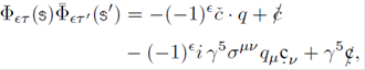 (18)
(18)
with the four-vectors  +
+
 )/2.
)/2.
The expansion of the operator Φϵτ ()'),
for 𝜖 = 𝜖', can be obtained with the operator γ5. After multiplying the first
equation in (10) by γ5, the energy effectively changes its sign but, the
eigenvalue for the spin equation keeps its sign
 (19)
(19)
Notice that, up to an unphysical phase, the operators (18) transform under γ5 as
 (20)
(20)
It is important to note that Eqs. (13), (18) and (B.1) (see Appendix B) have no arbitrary phases; this is relevant when one is interested in the relative phases of a multiparticle process.
As an elementary application of expressions (13) and (18), the transition amplitude for a vector operator Γ = 𝜐𝜇γ𝜇 and for spinors with the same energy sign is shown in Appendix B. However, by using the formulas (13), (A.1), (18), and (20), it is possible to perform calculations for any kind of transition amplitude with a systematic methodology. Nevertheless, this is a special case of the more general projective method.
3.2. General projective method
When one deals with an analytic amplitude calculation, like the one in equation (13), the implementation of a specific basis is useful to optimize the overall procedure. Particularly, the rest basis is a powerful tool to obtain the spin-dependent amplitude. A specific interaction term Γ could be successfully treated with a suitable election of the spinorial basis. Such a basis will be used in the generalized formula (13)
where the spinors 𝜔r (Q, S) were defined above and the notation of the spin-energy projectors are used, with
Formula (21) reflects the main idea of this work. Although it is written with a general basis, it shows formidable characteristics of the completeness of a spinorial basis, i.e., the reduction of the amount of work needed, and the explicit covariance of the expressions obtained. Instead of working with the squared modulus of the amplitude |M|2, formula (21) allows one to deal with the transition amplitude M itself, without invoking non-physical quantities, and using a decomposition of the original transition amplitude in terms of elementary amplitudes
4. The massless-spinor method
Any massive spinorial basis possesses the interesting symmetry provided by the operator γ5. Multiplying Eqs. (3) by γ5 shows that the spinors γ5ωr (Q, S) are also its solutions. Actually, the spinor γ5 ωr (Q, S) corresponds to an energy sign -Kr and spin sign -𝛿r as follows
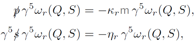 (23)
(23)
where K r = +1, 𝜂 r = +1 for r = 1, 2 and K r = -1, 𝜂 r = -1 for r = 3,4. This is a consequence of the PCT transformation over the spinor part of the wave functions (2). Nothing prevents the use of the set of eight linearly dependent massive spinors {𝜔 r (Q, S), γ 5 𝜔 r (Q,S)} as an over-complete basis.
There are multiple ways to reduce this set to a complete basis. For example, the linear combinations 𝜔 r (Q,S) ± γ 5 𝜔 r +2(Q, S), with r = 1, 2, form a complete basis. How ever, some useful linear combinations are
with λ = ±1. The eight states (24) are not anymore eigen-states of Eqs. (3), but they fulfill
and, with an appropriate phase selection, have the nontrivial orthogonality properties
Equations (24), (25) and (26) suggest that a decomposition of the massive spinor space into two complementary spaces can be made. This approach emerges when one reinterprets equation (24) as the result of projecting the state 𝜔 r (Q,S) with the chiral projector operators ρλ = (1 + λγ 5)/2. Effectively, an operator O can be decomposed into the direct sum of two operators, which are acting, separately, on the ρλ and ρ-λ subspaces. This can be seen explicitly in each splitting of the covariant operators
and it means that two independent bases can be constructed in each of these subspaces.
A general eigenstate of Eq. (25) can be dentoed as
where k2 = (ζ k0)2
-
As a consequence, a basis will be formed by spinors
where we have used the normalization of the states (24); this implies that the expansion of any operator in each subspace will be
The different λ signs in the spinors in expression (30) are required by expression (29). This is an evidence that both, an operator O (acting over the four-dimensional spinor space) and a spinor 𝜔
r
(Q, S), need the four Weyl spinors
Then, a covariant expression for the expansion of any spinor w in terms of Weyl spinors is
where 𝜔 can be a massive or massless spinor.
Equation (31) is useful to select a complete basis from the eight states (24) but, as can be seen, there is no unique way to form a complete basis using states (24). Equation (28) helps in the task. The combination of the dynamical quantities k t = p + t m s, with t = ±1, are two, nonorthogonal, light-like four-vectors. k/t on the states (24) yields
 (32)
(32)
A remarkable property of the operators  t is shown by the right-hand side of the Eq. (32). Imposing the condition k
r
-𝜆t𝜂r = 0, it is possible to establish a Weyl-like equation over the states (24).
t is shown by the right-hand side of the Eq. (32). Imposing the condition k
r
-𝜆t𝜂r = 0, it is possible to establish a Weyl-like equation over the states (24).
For example, if we explicitly choose the basis +1, while the others, -1. Other selections can be found, for example, in [?]. We can change the label (R) → R and then, the orthogonality rules among them reduce to
The expansion of an arbitrary, massive or massless, spinor 𝜔 can be written as
As a first elementary application of formula (34), we present the massive spinors in terms of massless spinors
where the same dynamical quantities Q = p, S = s have been used in formula (34); this means that
with ρ = r + 𝜅
r
- 1, and
Having established the connection with the massless spinor basis, now we will study the helicity formalism relation with the formalism of this work.
5. Helicity-spinor method
5.1. Helicity amplitude
An helicity spinor [36]

with Σ k = 𝜖 klm σ lm ,the helicity sign h ± 1, and helicity-spin four-vector
It is essential to be careful with the noncovariant appearance of the second Eq. (37). This equation can be translated to the apparently covariant expression
where both Eqs. (37) are involved in its deduction. For Lorentz-boost transformations that do not reverse the direction of
It is useful to define the helicity associated rest basis of a helicity spinor
The correspondence between the bases
where the notation
The elements
with 𝜖 = (3 - 𝜅) /2 and 𝜏𝜅h = (3 - 𝜅h)/2.
Formula (40) can be used to express a general spinor 𝜔 r (Q, S) in terms of the helicity associated rest basis
where the helicity spinorial basis
In the next section an elementary use of the formulas developed in Secs. (3-5) is presented. There, multiple expressions for the amplitude of the Compton process are derived.
6. An example: the Compton effect
The transition amplitude for the Compton process (see Fig. 1) is

 (45)
(45)
where
Using the Mandelstam variables
and after some manipulations, one can rewrite equation (45) as
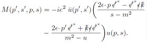 (47)
(47)
The use of the equation  u(p, s) = mu(p, s), the four-momentum conservation p + k = p
'
+ k
'
and the gamma matrices identity γ
α
γ
β
γ
δ
= 9
αβ
γ
δ
- g
αδ
γ
β
+ 9
βδ
γ
α
+ ίε
αβδμ
γ
5
γ
μ
, reduces the number of gamma matrices. If the final terms are arranged, expression (47) looks as
u(p, s) = mu(p, s), the four-momentum conservation p + k = p
'
+ k
'
and the gamma matrices identity γ
α
γ
β
γ
δ
= 9
αβ
γ
δ
- g
αδ
γ
β
+ 9
βδ
γ
α
+ ίε
αβδμ
γ
5
γ
μ
, reduces the number of gamma matrices. If the final terms are arranged, expression (47) looks as
 (48)
(48)
where
Using the spinor techniques, and the compact expression (48), efficient treatment of the amplitude can be made as it is shown below.
6.1. The helicity-spinor method
With formulas (18) and (42), the helicity amplitude for this process is
Equation (51) explicitly shows three parts: kinematic elements through the hyperbolic functions, the spin direction elements
Using expressions (48), (49), (50) and formula (C.1), the amplitude for general spin directions is
with
and
6.2. The massless-spinor method
Using equations (34) and (36), the transition amplitude is
As stated above, it is easy to obtain expressions for
where
where
6.3. The projective method: The rest basis
Because this formula is too long, it can be found in Appendix D.
6.4. The projective method: Using the Lorentz-invariant property of the amplitude
The amplitude (48) is a Lorentz scalar and it allows us to compute its analytical value in the reference frame where the electron is initially at rest. The result is general because it is possible to rewrite all the variables in another frame using a Lorentz transformation. With the aid of equation (21) and the covariance of amplitude (48), we get
The (two-component) spinors 𝜙', 𝜙 have their spin quantization directions defined by the
final  and
initial spin
three-dimensional vectors in their respective rest frames. The notation for a
and
and
initial spin
three-dimensional vectors in their respective rest frames. The notation for a
and
where we have used the radiation gauge
7. Conclusions
The notion of covariant-spinorial operator helps to understand the importance of massive spinors' closure property. An important consequence of this is shown by Eq. (6). Although we do not take advantage of this equation, Eq. (6) clarifies the arguments that are employed in the text. It shows the origin of the covariance and generality of our results.
Our procedure, the projective method, allows computing transition amplitudes using a decomposition of a (massive or massless) spinor as a linear combination of others (massive or massless) spinors which, in principle, are not related to the problem. However, to avoid unnecessary phases, it is helpful to use a spinorial basis related to the problem.
We have shown that most common spinor techniques, as the helicity- and massless-spinor methods, can be formulated using the idea of a complete spinorial basis. This framework allows us to exploit the symmetries and properties of the spinors, without the need for a specific representation for them or for the gamma matrices, allowing a wider understanding of the formalism. The framework thus proposed is free of unphysical singularities, therefore it could be fruitful to implement it within a computational code.
For instance, the spinorial basis at rest allows for obtaining closed formulas, which are fully covariant, for transition amplitudes. Thus, without requiring a particular four-component spinor representation and with no need to fix arbitrary phases. The use of this particular basis is a great example of how spinor symmetries help on the obtaining of useful formulas; at the same time, it permits to get analytical values of any amplitude using, simultaneously, two or more different bases. This is relevant, particularly if one has an interest in evaluating the efficiency, or shortcomings, of different schemes, like those related to singularity issues in the amplitude.
As an example of our procedures, formulas for the Compton amplitude, for helicity states and general spin states, were obtained. It can be noted that Eq. (51) has not been computed for a particular frame as our procedure does not depend on such an election. Also, the structure of Eq. (51) shows separately the kinematic, spin direction and dynamical factors, which are useful in the analysis of any process. The covariance of the framework is exploited with the formula (58), a compact expression for general spin configurations. It could be useful studying polarization effects, such as the electron spin asymmetry using polarized photons, or the photon helicity asymmetry using unpolarized electrons.

